
Multi-level Latency Evaluation with an MDE Approach
Daniela Genius
1
, Letitia W. Li
2,3
, Ludovic Apvrille
2
and Tullio Tanzi
2
1
Sorbonne Universit
´
es, UPMC Paris 06, LIP6, CNRS UMR 7606, Paris, France
2
LTCI, T
´
el
´
ecom ParisTech, Universit
´
e Paris-Saclay, 75013, Paris, France
3
Institut VEDECOM, 77 Rue des Chantiers, 78000 Versailles, France
Keywords:
Embedded Systems, System-level Design, Simulation, Virtual Prototyping, Latency.
Abstract:
Designing embedded systems includes two main phases: (i) HW/SW Partitioning performed from high-level
functional and architecture models, and (ii) Software Design performed with significantly more detailed mod-
els. Partitioning decisions are made according to performance assumptions that should be validated on the
more refined software models. In this paper, we focus on one such metric: latencies between operations. We
show how they can be modeled at different abstraction levels (partitioning, SW design) and how they can help
determine accuracy of the computational complexity estimates made during HW/SW Partitioning.
1 INTRODUCTION
Applications modeled at high levels of abstraction
contain a very indeterminate notion of latency. This
is typically the case for applications modeled in the
scope of system-level hardware / software partition-
ing. When applications are mapped onto virtual or
existing hardware, in particular onto multi-processor
systems-on-chip (MP-SoC), latencies become a func-
tion of multiple precise factors: cache effects, mem-
ory latencies, bus or network on chip transfers, syn-
chronization latency between processors.
TTool (Apvrille, 2008) supports both Partitioning
and System Design, and considers that partitioning
decisions may need to be changed due to additional
information from verifications performed during the
System Design phase. Recent work studied how to
feed back information such as cycles per instruction
and cache miss rate, but did not yet include latency
between operators nor a definition of a refinement re-
lation between abstraction levels (Genius et al., 2017).
We explain how latencies of these modeling lev-
els relate to one another, and how results can be back-
traced to models at higher abstraction levels e.g. from
software to partitioning models. We can thus gener-
ate hardware/software platform from models that can
be simulated at very low level. Our method is suited
to MP-SoCs with many processors and complex inter-
connections e.g. network on chip. Latency precision
increases as cycle and bit accurate levels take into ac-
count application, hardware and operating system.
Section 2 presents the related work. Section 3 fo-
cuses on our method. Section 4 explains the notion of
latency on different abstraction levels within an MDE
approach. Section 5 details the rover case study and
shows how latencies can be determined at different
levels. Section 6 concludes the paper.
2 LATENCIES IN RELATED
WORK
A number of system-level design tools exist, offering
a variety of verification and simulation capabilities at
different levels of abstraction.
Sesame (Erbas et al., 2006) proposes modeling
and simulation features for MP-SoC at several ab-
straction levels. Semantics vary according to the level
of abstraction, ranging from Kahn process networks
(Kahn, 1974) to data flow for model refinement, and
discrete events for simulation. Sesame is however
limited to the allocation of processing resources. It
models neither memory mapping, nor the choice of
the communication architecture, and is thus less pre-
cise than tools including these aspects.
The same research team proposes the Daedalus
(Thompson et al., 2007) design flow, which allows to
evaluate latencies at a register transfer level. Daedalus
is however targeted towards automated synthesis
of multimedia streaming applications on MP-SoC,
which are somewhat more predictable than typical
Genius, D., Li, L., Apvrille, L. and Tanzi, T.
Multi-level Latency Evaluation with an MDE Approach.
DOI: 10.5220/0006535902950302
In Proceedings of the 6th International Conference on Model-Driven Engineering and Software Development (MODELSWARD 2018), pages 295-302
ISBN: 978-989-758-283-7
Copyright © 2018 by SCITEPRESS – Science and Technology Publications, Lda. All rights reserved
295

embedded applications that interact with the environ-
ment in many ways. SATURN (Mueller et al., 2011)
uses Artisan Studio (Atego, 2017) for SysML editing
and performs a co-simulation using the QEMU soft-
ware emulator. It can also configure an FPGA. How-
ever, simulations under SystemC are performed only
at the quite high TLM-2.0 abstraction level (OSCI,
2008) which makes latency measurements less pre-
cise.
The Architecture Analysis & Design Language
AADL allows the use of formal methods for safety-
critical real-time systems, with a focus on latency and
safety, properties which are also important in the con-
text we explore. Similar to our environment, a pro-
cessor model in AADL can have different underly-
ing implementations and its characteristics can easily
be changed at the modeling stage (Feiler and Gluch,
2012).
MARTE (Vidal et al., 2009) shares many com-
monalities with our overall approach; however, it
lacks separation between control and message ex-
change. More recent work (Taha et al., 2010) con-
tains hardware platform generation and support sim-
ulation using Simics, a full-system simulator; origi-
nally purely functional, il now permits cycle-accurate
simulation. A binary of the software is loaded onto
the platform, and runs under an operating system.
The work shown in (Lee et al., 2008) uses a
UML/MARTE model to express AADL flow laten-
cies and takes into account worst case latencies and
jitter. This work is more (but not exclusively) focused
on the periodic case and does not contain a virtual
prototyping phase.
MDGen from Sodius (Sodius Corporation, 2009)
generates SystemC code from SysML models. It
adds timing and hardware specific artifacts such as
clock/reset lines to Rhapsody models and generates
synthesizable, cycle-accurate implementations. In
these aspects, it is very similar to our tool, which gen-
erates a cycle and bit accurate simulation platform;
MDGen however does not fully address correctness
by construction aspects.
The B method and more recently Event-B (Abrial,
2010) model systems at different abstraction levels
and mathematically prove consistency between re-
finement levels. Based on set theory and the B
language, it is well established in large-scale pub-
lic/private projects (urban transports etc.) but much
less widespread in industry than UML/SySML based
approaches.
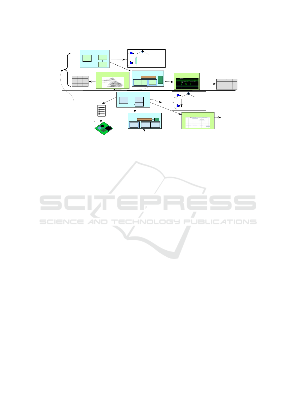
3 METHODOLOGY OVERVIEW
Our methodology for the design of embedded systems
involves design at four levels of abstraction where dif-
ferent latency measurements (see Figure 1).
The Partitioning Level features two sub-levels.
1. The purely functional level relies on logical time,
where latency is based on the logical time be-
tween functional operators describing the behav-
ior of tasks. These operators can describe non de-
terministic behavior, and model in an abstract way
the complexity of computations.
2. The system-level mapping level gives a physical
time to complexity operations, thus giving a phys-
ical time to latencies. However, the high level ab-
stract hardware components of our approach make
these latencies imprecise: the values we obtained
– which might be used as a partitioning decision –
are meant to be confirmed during the next levels.
The Software Level also includes two sub-levels.
1. At the software design level, software is mod-
eled with blocks and state machine diagrams. The
transitions between states can be annotated with
minimum and maximum physical time functions
(after, computeFor). Latency estimates between
states/transitions are obtained by interactive sim-
ulation, without any hardware model.
2. The deployment level allows a designer to map
software blocks onto hardware elements (CPU,
memory, etc.). A cycle and bit accurate SystemC-
based simulation is then used to obtain a cycle-
precise measurement of latencies. Latencies ob-
tained there can be used to correct decisions (e.g.
partitioning decisions) taken at the higher level
(e.g., at system-level mapping).
4 LATENCIES IN MDE
In this section, we formally define latencies with re-
gards to their abstraction levels.
4.1 Latencies
We assume a model M = (T,Comm), which contains
a set of execution elements (Tasks) and communi-
cations between tasks. T can be defined as T =
(Op, n) with Op being a set of operators - control,
communication, complexity - and n a next function
n : op 7→ {op
0
} returning all the subsequent operators
of a given operator. A complexity operator is an op
that abstracts a computation into either a number of
MODELSWARD 2018 - 6th International Conference on Model-Driven Engineering and Software Development
296
Functional Level
Partitioning
Software
Design
Task1
Task3
Task2
Behavior
Model
Operator1
Complexity
Operator2
...
Abstract Hardware Components
Logical Time
Latency
Mapping Level
Task3 Task1
Task2
Physical Time
Reachability Graph
Execution trace
Min, Max Latency
Min, Max,
Average Latency
Execution
Traces
Software Level
Task1'
Task2_1
Task2_2
Behavior
Model
Operator1'
Time Function
Operator2'
...
Latency
Code Generation
Reconsideration
of Partitioning
Model if
significant
discrepancies in
corresponding
latencies
Deployment Level
Virtual Prototyping
Precise simulation → Precise latencies
Execution
on Target
Task1' Task2_1 Task2_2
Simulation (no HW)
Formal Verification
Simulation
Estimated
Latencies
Figure 1: Latency Measurement through the Embedded System Design Process.
operations to be executed or a physical time. Also,
an operator op that belongs to a task t of a model M
is denoted op
M,t
. An execution environment is de-
noted as E = (M, H, m
t
, m
c
) where M is a model, H
a set of hardware nodes, m
t
a function mapping tasks
to executions nodes of H and m
c
a function mapping
communications to communication and storage nodes
of H.
4.1.1 Computing Latencies
Occurrences O of an operator op
1
of an execution
of t ∈ T are expressed as the set of all times x of op
1
:
O(op
1
) = {x
op
1,1
, x
op
1,2
, . . . }.
We can thus determine for a given E the set of all la-
tencies L
E
op
1
,op
2
between op
1
and op
2
, where for each
x
op
1
∈ O(op
1
), we find the first occurrence of op
1
af-
ter each occurrence of op
2
, calculated as the mini-
mum of all x
op
2
∈ O(op
2
) where x
op
2
> x
op
1
. Then,
we can define the min latency as:
l
E
min;op
1
,op
2
= min(L
E
op
1
,op
2
).
Similarly, the max and mean can be defined.
4.1.2 Correspondence between Latencies
Our objective is to be able to relate latencies of mod-
els at different abstraction levels so as to confirm de-
cisions taken at the highest abstraction level. To relate
latencies, we first need to relate operators of different
abstraction levels. We thus define a correspondence
relation between operators of two abstraction levels u
(for upper) and l (for lower). C (op) is therefore de-
fined as:
∀op
M
l
,t
l
, noted op
l
, C (op
l
) =
op
u
φ otherwise
We can thus relate latencies when op
l,1
and op
l,2
of M
l
have both a non empty correspondence in M
u
.
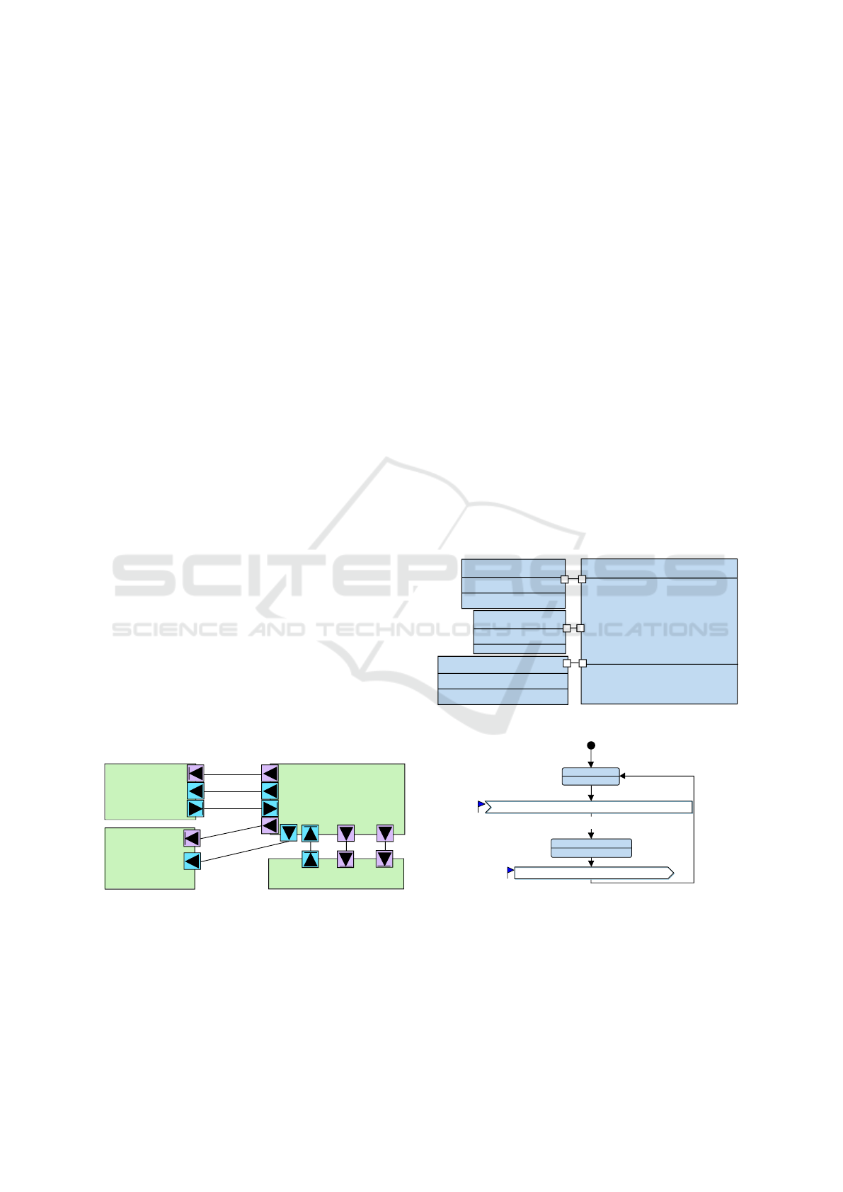
Figure 2 explains how latencies and models relate
across different abstraction levels. Since the goal is
to relate operators of functions and blocks, we do not
need R to be a refinement relation between the exe-
cution environments E
u
and E
l
. Therefore, the engi-
neer is in charge of ensuring that hardware nodes have
been correctly refined, and mapping relations adapted
to the refined model.
R can be defined as follows. Tasks can be split
in subtasks. Complexity operators can be replaced
by a sub-behavior. Communications between tasks
may be added in order for subtasks to exchange in-
formation, but communication operators can only be
added in sub-behaviors replacing complexity opera-
tors. More formally, if M
u
= (T
u
,Comm
u
) with ∀t ∈
T
u
, t = (Op
u
, n
u
), then t can be refined by R :
1. t
u
can be replaced by k tasks t
1,l
,t
2,l
, . . . ,t
k,l
with
k > 0 and Op
u
∈ ∪Op
x,u
i.e. the operators of t
u
are
split among the k tasks if k > 1, then additional
communications and controls may be introduced
between operators of the original tasks, thus pro-
voking an update of next functions n
l
in the lower
levels.
2. Each complexity operator can be replaced by a
sub-behavior:
Op
u
= (O
u,ctrl
, O
u,comm
, O
u,complexity
, O
u,sub
).
A sub-behavior Sub = (Op, n, n
r
) can be seen as
a sub-activity of the main task that suspends the
main task when it is triggered, and that has a next
operator n
r
that resumes the task to the corre-
sponding next operator in the main task. There-
fore, the n function of a sub activity must refer-
ence only operators of this sub activity.
Let us now apply the latency concepts to our ab-
stractions levels: partitioning, and software design.
Multi-level Latency Evaluation with an MDE Approach
297

M
u
E
u
(M
u
, H
u
, mt
u
, mc
u
)
Models
Execution env.
Upper
abstraction
level
Lower
abstraction
level
M
l
E
l
(M
l
, H
l
, mt
l
, mc
l
)
C
R
l
Eu
u,min/max/mean, opl1, opl2
l
El
l,min/max/mean, opl1, opl2
op
u1
op
u2
op
l1
op
l2
Figure 2: Relations between models and latencies between
two abstraction levels.
4.2 Partitioning
The HW/SW Partitioning phase of embedded system
design models the abstract, high-level functionality
and architecture of a system (Knorreck et al., 2013).
It follows the Y-chart approach, first modeling the
abstract functional tasks, candidate architectures,
and then finally mapping tasks onto the hardware
components (Kienhuis et al., 2002). The application
is modeled as a set of communicating tasks on the
Component Design Diagram (an extension of the
SysML Block Instance Diagram). Task behavior is
modeled using control, communication, and compu-
tation operators.
A Partitioning P is defined as a set of models P =
(FM, AM, MM), with FM a Functional Model, AM
an Architecture Model, and MM a Mapping Model.
4.2.1 Functional Level
A Functional Model is defined as FM = (T,Comm)
when T is a set of Tasks, and Comm is a set of Com-
munications between tasks. A Task t is defined as
t = (Attr, B) with Attr a set of Attributes, and B a be-
havior.
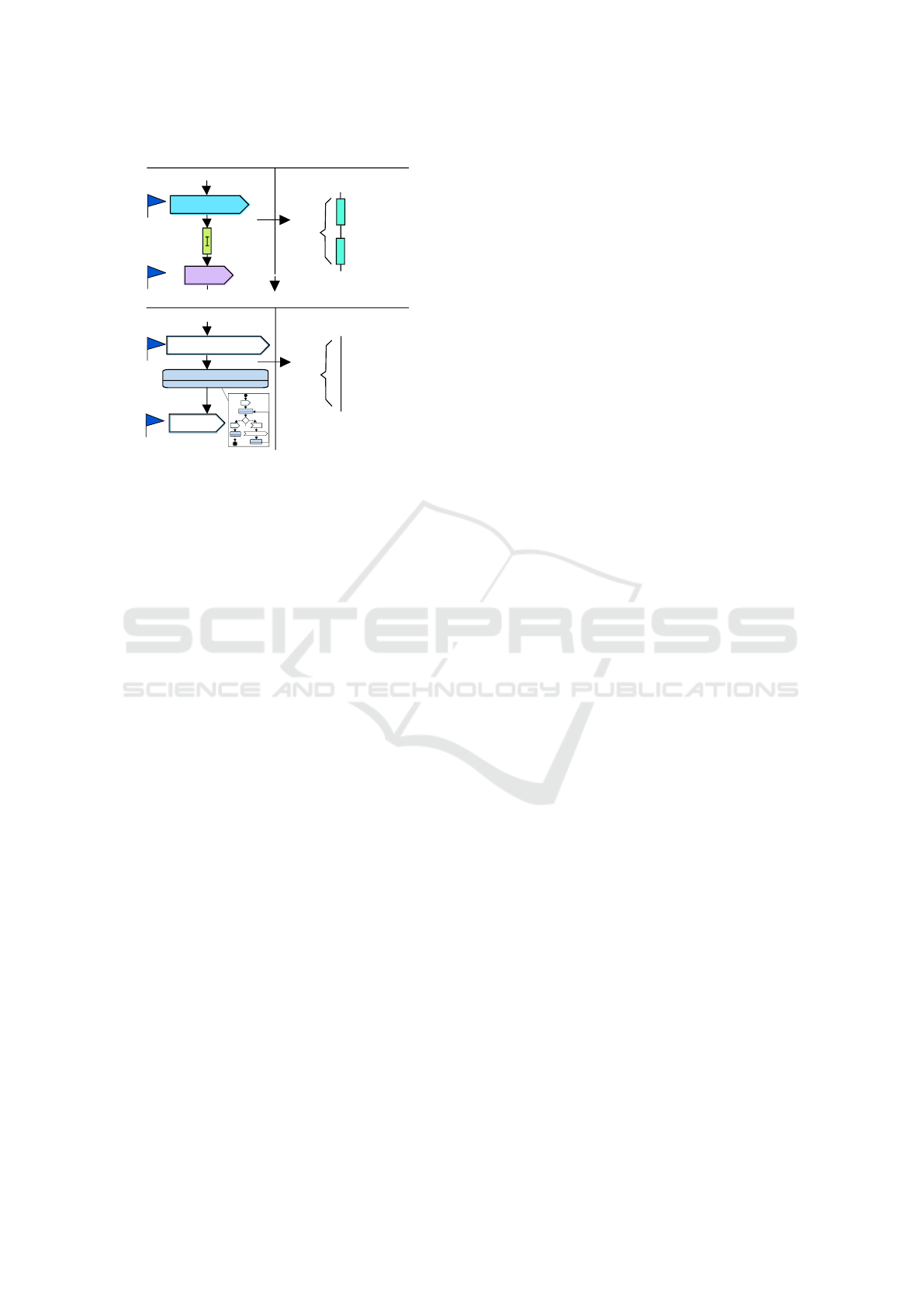
The Behavior B = (Ctrl,CommOp,CompOp)
consists of Control Operators Ctrl – such as loops,
choices, etc. – Communication Operators CommOp
– channel read/write, events send/receive – , and
Complexity operations CompOp, who model the
complexity of algorithms through the description of
a min/max interval of integer/float/custom operations
on an execution hardware (CPU, hardware accelera-
tor, FPGA, etc.), see the top left part of Figure 3.
At this abstraction level, latency is defined as
the logical time between complexity operators as
shown in Figure 1.
4.2.2 Mapping Level
Mapping involves allocating tasks onto the architec-
tural model. A task mapped to a processor will be im-
plemented in software, while a task mapped to a hard-
ware accelerator will be implemented in hardware.
The architectural model is a graph of execution
nodes (CPUs, Hardware Accelerators), communica-
tion nodes (Buses and Bridges), and storage nodes
(Memories). Hardware components are highly ab-
stracted: a CPU is defined as a set of parameters such
as an average cache-miss ratio, go idle time, context
switch penalty, etc. An Architecture Model
AM = (CommNode, StoreNode, ExecNode, link)
is built upon abstract Hardware Components: Com-
munication Nodes CommNode, Storage Nodes
StoreNode, Execution Nodes ExecNode, and archi-
tectural links between Communication Nodes and any
other node link. ExecNode defines a conversion
from Complexities to Cycles, and a speed convert-
ing Cycles to seconds. Similarly, CommNode and
StoreNode give a physical time to logical transac-
tions. The mapping therefore specifies a physical
time for latencies defined at functional level, as
shown by the top right part of Figure 3.
We can determine latencies in physical time in two
different ways.
1. A Formal Verification FV : P → RG is a function
that takes as argument a Partitioning P and outputs
a Reachability Graph RG. RG contains all pos-
sible Execution Traces ET . The analysis of RG
makes it possible to obtain minimum and maxi-
mum latency values i.e. l
P
min
and l
P
max
.
2. Less formally, a simulation of P generates one sin-
gle Execution Trace, in which we can measure the
minimum, maximum, and average latencies be-
tween any given two operators during that single
execution trace: l
P
min
, l
P
max
and l
P
mean
4.3 Software Design
A software design consists of both a software model,
and a experimentation of this software running on a
(virtual) prototype.
4.3.1 Software Model
A Software Design model can be considered a
refinement of a Partitioning model, where only
software-implemented tasks are modeled with their
detailed implementation, thus realizing the R re-
lation: some tasks of P might be split while extra
communications related to split tasks can be added.
Figure 3 shows the relation of Behavior Models
between Partitioning and Software Design models.
MODELSWARD 2018 - 6th International Conference on Model-Driven Engineering and Software Development
298
sig()
state0
sig()
sig()
state1
state2
Partitioning
Before mapping
evt
event()
chl
channel(size)
Algorithm
Complexity
Channel Operator
After mapping
Channel
Transit
Time
Algorithm
Execution
Time
Event Operator
Latency
Software Design
Channel Signal Operator
Channel
Time
Function
Algorithm
Time
Function
Event Signal Operator
Latency
Modeling
Execution on Target
calculateAlgorithm
signal1(attribute)
signal2()
Figure 3: Relation between latencies in Partitioning and
Software Design Models.
The Software Model S = (T, I) can also be defined
as a set of Tasks t and Interactions i between tasks.
Regarding the behavior of tasks, while Partitioning
models express algorithms as an abstract complex-
ity operation and communications in terms of their
size only, Software Design models describe the im-
plementation of algorithms with a sub-behavior de-
scription using attributes, and interactions (based on
signals exchanges) contain exchanged values stored
in attributes of blocks. Thus, the set of attributes of
software tasks is likely to be enriched both with re-
gards to the partitioning model for algorithms details
and communication details.
Furthermore, the complexity operators in Parti-
tioning, expressed as a function of execution cycles,
are translated into either a time function T F() or sub-
behavior subB. More formally, the transformation re-
lation of partitioning behavior to software design be-
havior can be expressed as:
B
P
= (Ctrl,Comm,Comp) →
B
S
= (Ctrl
0
,Comm
0
, T F, subB)
thus following the approach explained in section
4.1.2. For those tasks present in both Partitioning and
Software Design models, while their behaviors ap-
pear different, their overall functionality should be the
same; traces of their execution flow should involve the
same sequence of operations and complexities/times.
If the complexities are accurate and the model cor-
rectly translated, measured latencies between corre-
sponding elements should remain the same.
Concerning latencies pertaining to communica-
tions, we restrict our analysis to those that remain un-
changed between levels. If significant discrepancies
occur, then there is an error in one of the models. The
computation complexities for certain algorithms may
have not been well estimated. Also, there could be an
inaccurate modeling of the architecture, with a CPI
(cycles per instruction) parameter not correctly set.
The formalizations introduced before provide a
correspondence function C which takes as input an
operator of a Software Design (lower level) and out-
puts an operator of the upper level (e.g., partitioning):
it can thus be used to relate latencies between soft-
ware design and partitioning models.
To find each corresponding Partitioning operator
op
P
for a Software Design operator op
SD
, we must
first determine if op
SD
was part of the subB added
during the refinement of a complexity operator. If so,
we conclude there is no corresponding operator op
P
.
If not, and the communication exists in both Software
Design and Partitioning, then we find the partitioning
operator that was translated into op
SD
during the re-
finement process.
The software model can be functionally simu-
lated, taking into account temporal operators but
completely ignoring hardware, operating systems and
middleware. This simulation aims to identify log-
ical modeling bugs, and estimate latencies, but the
real computation of latencies (min, max, mean) is ex-
pected to be performed with the Software Prototyping
execution model.
4.3.2 Software Prototyping
In order to prototype the software components with
the other elements of the destination platform (hard-
ware components, operating system), we use a
so-called Deployment Diagram in which tasks are
mapped to a model of the target system. Then, a
model transformation generates the software elements
(tasks, main program) and the hardware elements
are built from the deployment information e.g. top
cells of the hardware components in SoCLib (So-
cLib consortium, 2003). The latter is an open li-
brary of multiprocessor-on-chip components based on
the shared memory paradigm, consisting of SystemC
models of hardware modules and an operating sys-
tem. Precise cycle and bit accurate models for the
hardware allow to measure the latency in terms of
simulation cycles.
In order to evaluate latencies when the system is
running, we proceed by intercepting the traffic on
the interface between interconnect and memory bank,
which has minimal impact on performance as it does
not increase the code size. The trace thus obtained
can then be analyzed to obtain latency values.
Multi-level Latency Evaluation with an MDE Approach
299
5 CASE STUDY
Autonomous vehicles and other robots have been pro-
posed for disaster relief efforts. Our case study de-
scribes the design of a rover, a small autonomous ve-
hicle which will search through rubble for disaster
victims. The rover is equipped with telemetric sen-
sors, located in the front, rear, top, and sides. These
sensors allow the rover to detect obstacles and nav-
igate the terrain autonomously (Tanzi et al., 2016).
The rover adjusts its acquisition behavior based on the
situation. When it detects no obstacles in proximity,
the rover decreases its sampling rate, assuming that
no obstacles will suddenly appear in its path. When
an obstacle is detected in close proximity, or within
its “safety bubble”, the rover adapts its behavior and
increases its rate of acquisition. When the rover has
detected obstacles in very close proximity, exact dis-
tances to obstacles become more critical.
Precise distance calculations depend not only on
the telemetric sensor measurements, but also on am-
bient conditions. Therefore, to obtain an exact mea-
surement, temperature and pressure sensors can be ac-
tivated. The rover must be able to respond to obstacles
within a set time frame – i.e., a maximal latency – to
avoid collisions.
5.1 Functional and Partitioning Levels
We begin by modeling at the partitioning level using
TTool’s DIPLODOCUS environment. The rover con-
sists of a main controller which receives data from a
distance sensor and temperature sensor, which it uses
to determine motor commands sent to the motor con-
trol, as shown in Figure 4. The main controller behav-
ior and sampling rate of the distance sensor depends
on the proximity of an obstacle (far away, intermedi-
ate, close).
MainControl
+ state : Natural;
+ calculateTraj : Natural;
+ calculateDistance : Natural;
DistanceSensor
TemperatureSensor
+ samplingRate : Natural;
+ sensorOn : Boolean;
MotorControl
startTemp
tempData
ultrasonicData
samplingRate
changeRate
motorCommand
newCommand
stopTemp
Figure 4: Rover Functional Model.
For simplicity, we map all tasks on one proces-
sor and all data transfer on one bus and one memory.
The mapping of tasks for our case study should en-
sure that the maximum latency between the detection,
decision and the resulting actions occurs within a re-
quired time frame. Latency checkpoints, represented
by small blue flags, are inserted at important points
in each component’s activity, such as on channel data
transfers which relay the sensor data to the main con-
troller and command transfers controlling the motor
(Figure 4).
• Temperature sensor data (written by Temperature-
Sensor, read by MainControl)
• Distance sensor data (UltrasonicData written by
DistanceSensor, read by MainControl on three
different paths
• Motor command (written by MainControl on
three different paths, read by MotorControl)
We moreover evaluate the latency between reception
of a signal of the DistanceSensor and a reaction via
motorCommand. We sssume the rover moves at 6
km/h, thus covering a distance of 100 meters per
minute. To determine the maximum latency between
two checkpoints, we use the interactive simulation of
TTool. Minimal, maximal and average latencies as
well as the standard deviations are determined for the
paths that were taken (left part of Table 1).
5.2 Software Design
<<block>>
MainControl
- state : int;
- sensorOn : bool;
- newRate : int;
- samplingRate: int;
- temp : int;
- leftVelocity: int;
- rightVelocity : int;
- distanceLeft : int;
- distanceRight : int;
- distanceFront : int;
~ out motorCommand(int leftVelocity, ...)
~ out control(bool sensorOn)
~ in tempData(int temp)
~ in ultrasonicData(int distanceLeft, ...)
<<block>>
DistanceSensor
- samplingRate : int;
- distance : int;
~ out ultrasonicData(...)
~ in changeRate(int samplingRate)
<<block>>
TemperatureSensor
- sensorOn = false : bool;
- temp : int;
~ in control(bool sensorOn)
~ out tempData(int temp)
<<block>>
MotorControl
- rightVelocity : int;
- leftVelocity : int;
~ in motorCommand(...)
Figure 5: Software Model with a SysML Block Diagram.
motorCommand(leftVelocity, rightVelocity)
sendMotorCommand
startController
ultrasonicData(distanceLeft, distanceFront, distanceLeft)
after (tsmin,tsmax)
computeFor (tcmin,tcmax)
computeFor (t1,t2)
calculation of
motor command
Figure 6: State machine diagram of MainControl.
5.2.1 Software Model
Figure 5 shows the tasks of the rover modeled us-
ing TTool’s Software/System Design environment,
AVATAR. There are four blocks corresponding to the
fours tasks already present in the functional model in
MODELSWARD 2018 - 6th International Conference on Model-Driven Engineering and Software Development
300
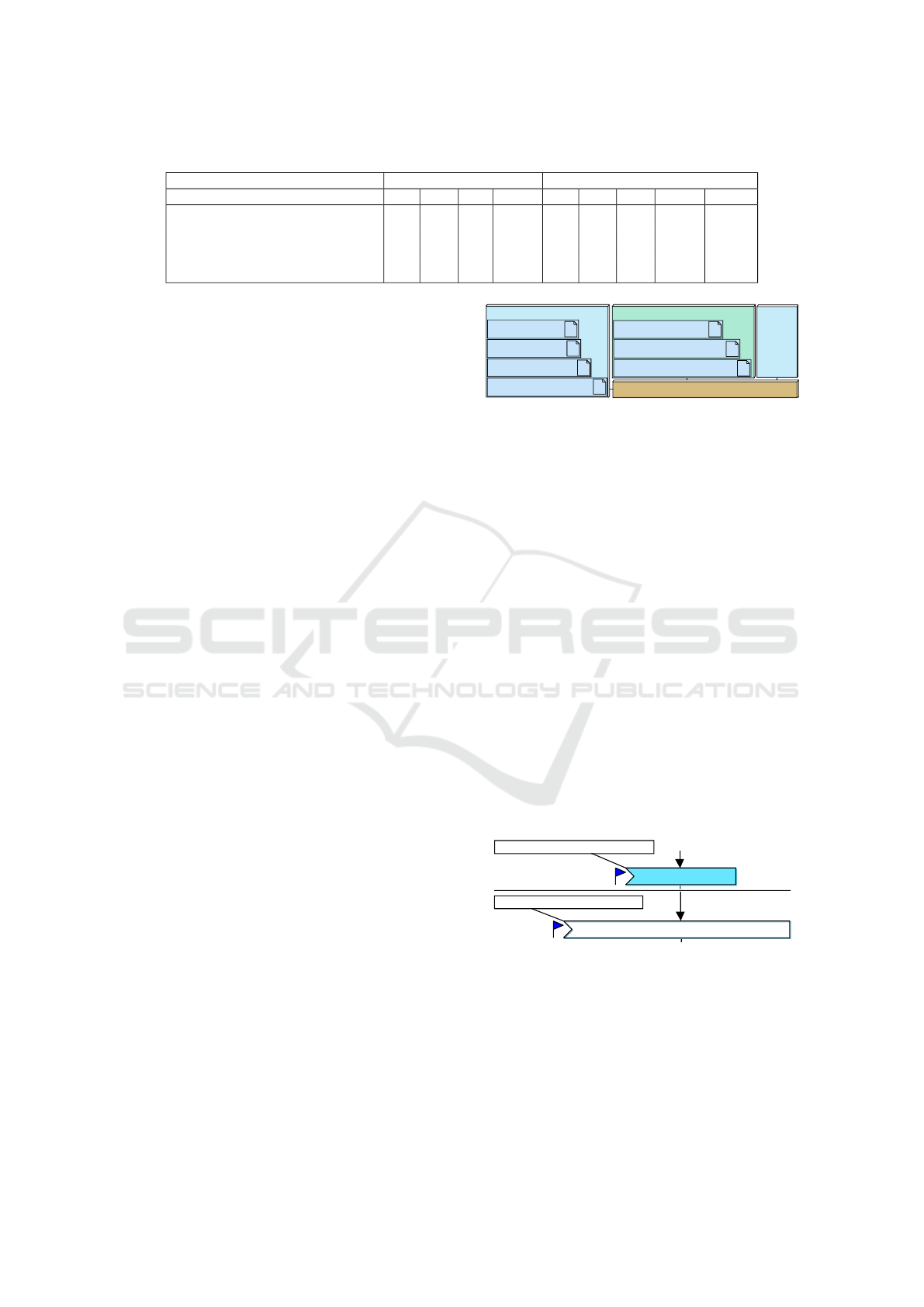
Table 1: Latencies.
Signal Partitioning level Software design level
min max avg std dev min max avg std dev SoCLib
s(tempData)-> r(tempData) 4 4 4 0 0 4 0.2 0.8 21.7
s(ultrasonicData)->r(ultrasonicData) 16 52 34 18 0 56 11.6 17.9 20.3
s(motorCommand)-> r(motorCommand) 5.7 10.3 8 2.3 0 16 4.9 3.3 32.3
s(ultrasonicData)-> r(motorCommand) 2 2 2 0 11 24 13.2 2.5 38.0
r(rultrasonicData)-> s(changeRate) 4 42 23 19 0 68 10.6 13.0 45.7
Figure 4. Figure 6 shows part of the the state ma-
chine diagrams of MainControl, leaving out the states
which compute the change of the sampling rate and
the motor control instructions. The two sensors with
their latency checkpoints and the data transmitted as
well as MotorControl closely resemble their higher-
level modeling counterparts. As a refinement on dis-
tance detection, we model left, front and right dis-
tances separately. MotorControl is essentially un-
changed, while temperature measurement simplifies
the stop and start events with a single control signal.
While the data transmitted through the chan-
nels is more precise than in the partitioning
model – for example, motorCommand now con-
sists of two integers leftCommand, rightCom-
mand, whereas ultrasonicData has three parame-
ters (distanceLeft,distanceFront,distanceRight, mo-
torCommand has two (leftVelocity, rightVelocity). On
the other hand, the main control automaton is simpli-
fied; branches can be taken depending on the data re-
ceived. Only five signals are required, regrouped into
three channels: from the viewpoint of mainControl,
two each for reception and control of data from the
distance and temperature sensors, and a last one for
motorControl.
5.2.2 Latency Evaluation
The right hand side of Table 1 shows the results we
obtained by performing an interactive simulation on
the software model (i.e. without any target platform),
examining as before the sensor data and motor control
channels as well as the latency between reception of
sensor data and sending of motor commands to deter-
mine if the reaction time is adequate. Again, the data
stemming from the DistanceSensor has a higher la-
tency and the differences between ultrasonicData and
tempData are even more important. The maximum
reaction time (last row) is higher, yet the rover con-
troller reacts on time to obstacles at least 3 cm away.
5.2.3 Software Prototyping
From the Rover Deployment Diagram (see Figure 7),
we generate the prototyping environment based on
SystemC top cells. In Figure 7, all tasks are mapped
<<CPU>>
CPU0
Design::MainControl
Design::DistanceSensor
Design::TemperatureSensor
Design::MotorControl
<<RAM>>
Memory0
MainControl/in tempData
MainControl/out motorCommand
MainControl/in ultrasonicData
<<VGSB>>
Bus0
<<TTY>>
TTY0
Figure 7: Rover Deployment Diagram.
onto one processor, and the three signals are mapped
onto one memory bank. For our experiments, we use
an instruction set simulator of a PowerPC 405 running
at a frequency of 800 MHz. The rightmost column of
Table 1 shows the results we obtain under SoCLib.
Latency variations on the prototype are much less
significant than those derived by interactive simula-
tion. In particular, the cost of a transfer of ultrasonic
data was overestimated in the Partitioning and Soft-
ware Models. On a MPSoC, using burst transfers, the
cost of transmitting several values is thus mostly over-
shadowed by the cost of the protocol.
5.3 Feedback of Latency Results
Latency requirements on channels are annotated by
the designer in the TTool diagrams. There are two
kinds of problems that can be detected after simula-
tion on the prototype and marked in the diagram: if
the simulation result at the current level does not meet
the requirement, or if it deviates more than a percent-
age fixed beforehand, we mark the label in red.
motorCommand(leftVelocity, rightVelocity)
sendSignal: motorCommand
4.9
chl
motorCommand(1)
writeChannel: motorCommand
8
Partitioning
Software design
Figure 8: Backtracing latencies.
Figure 8 shows the latency for a motorCommand
issued by MainControl and received by MotorCon-
trol. The boxes on the left denote that the signal ar-
rives from another block. We detect a deviation of
the latency for motorCommand on the software de-
sign level. Thus we can correct the assumptions on
the partitioning.
Multi-level Latency Evaluation with an MDE Approach
301

6 DISCUSSION AND FUTURE
WORK
This paper formalizes latency modelling and latency
measurements at different abstraction levels in an
MDE design flow. The principal contribution is the
establishment of a formal connection between the la-
tencies on the higher and lower levels of abstraction
followed by a validation by simulation of the soft-
ware part on a cycle-accurate model of a MP-SoC.
Our work makes it possible to detect incoherencies in
the models, backtrace results to the higher levels and
indicate when latency requirements are not met or di-
verge too strongly across different levels.
Our toolchain relies entirely on free software;
many others, also cycle-accurate, use commercial
SysML editors or simulation tools (Taha et al., 2010;
Mueller et al., 2011; Sodius Corporation, 2009).
The complete backtracing phase, also containing
information on cache miss rate, cycles per instruction,
etc., obtained at the lower levels, will be fully auto-
mated in the future, a step towards a complete multi-
level Design Space Exploration environment.
REFERENCES
Abrial, J.-R. (2010). Modeling in Event-B: system and soft-
ware engineering. Cambridge University Press.
Apvrille, L. (2008). TTool for DIPLODOCUS: an environ-
ment for design space exploration. In Proceedings of
the 8th International Conference on New Technologies
in Distributed Systems, pages 28–29. ACM.
Atego (2017). Artisan Studio. http://www.atego.com.
Erbas, C., Cerav-Erbas, S., and Pimentel, A. D. (2006).
Multiobjective optimization and evolutionary algo-
rithms for the application mapping problem in multi-
processor system-on-chip design. IEEE Transactions
on Evolutionary Computation, 10(3):358–374.
Feiler, P. H. and Gluch, D. P. (2012). Model-based engi-
neering with AADL: an introduction to the SAE archi-
tecture analysis & design language. Addison-Wesley.
Genius, D., Li, L. W., and Apvrille, L. (2017). Model-
Driven Performance Evaluation and Formal Verifica-
tion for Multi-level Embedded System Design. In
Confer
´
ence on Model-Driven Engineering and Soft-
ware Development (Modelsward’2017), Porto, Portu-
gal.
Kahn, G. (1974). The semantics of a simple language for
parallel programming. In Rosenfeld, J. L., editor, In-
formation Processing ’74: Proceedings of the IFIP
Congress, pages 471–475. North-Holland, New York,
NY.
Kienhuis, B., Deprettere, E., van der Wolf, P., and Vissers,
K. (2002). A Methodology to Design Programmable
Embedded Systems: The Y-Chart Approach. In Em-
bedded Processor Design Challenges, pages 18–37.
Springer.
Knorreck, D., Apvrille, L., and Pacalet, R. (2013). For-
mal System-level Design Space Exploration. Con-
currency and Computation: Practice and Experience,
25(2):250–264.
Lee, S.-Y., Mallet, F., and De Simone, R. (2008). Deal-
ing with aadl end-to-end flow latency with uml marte.
In Engineering of Complex Computer Systems. 13th
IEEE International Conference on, pages 228–233.
IEEE.
Mueller, W., He, D., Mischkalla, F., Wegele, A., Larkham,
A., Whiston, P., Pe
˜
nil, P., Villar, E., Mitas, N.,
Kritharidis, D., et al. (2011). The SATURN approach
to sysml-based hw/sw codesign. In VLSI 2010 An-
nual Symposium, pages 151–164, Lixouri, Greece.
Springer.
OSCI (2008). Osci tlm-2.0. www.accelera.com.
SocLib consortium (2003). The SoCLib project: An inte-
grated system-on-chip modelling and simulation plat-
form. www.soclib.fr.
Sodius Corporation (2009). MDGen for SystemC.
http://sodius.com/products-overview/systemc.
Taha, S., Radermacher, A., and G
´
erard, S. (2010). An
entirely model-based framework for hardware design
and simulation. In DIPES/BICC, volume 329 of IFIP
Advances in Information and Communication Tech-
nology, pages 31–42. Springer.
Tanzi, T., Chandra, M., Isnard, J., Camara, D., Sebastien,
O., and Harivelo, F. (2016). Towards ”drone-borne”
disaster management: Future application scenarios.
In ISPRS Annals of Photogrammetry, Remote Sensing
and Spatial Information Sciences, volume III-8, pages
181–189.
Thompson, M., Nikolov, H., Stefanov, T., Pimentel, A. D.,
Erbas, C., Polstra, S., and Deprettere, E. F. (2007).
A framework for rapid system-level exploration, syn-
thesis, and programming of multimedia MP-SoCs. In
Hardware/Software Codesign and System Synthesis,
pages 9–14. IEEE.
Vidal, J., de Lamotte, F., Gogniat, G., Soulard, P., and
Diguet, J.-P. (2009). A co-design approach for embed-
ded system modeling and code generation with UML
and MARTE. In Design, Automation and Test in Eu-
rope, pages 226–231, Dresden, Germany.
MODELSWARD 2018 - 6th International Conference on Model-Driven Engineering and Software Development
302
