Learning to Evaluate Chess Positions with Deep Neural Networks and

Limited Lookahead

Matthia Sabatelli

1,2

, Francesco Bidoia

, Valeriu Codreanu

and Marco Wiering

Monteﬁore Institute, Department of Electrical Engineering and Computer Science, Université de Liège, Belgium

Institute of Artiﬁcial Intelligence and Cognitive Engineering, University of Groningen, The Netherlands

Surfsara BV, Science Park 140, Amsterdam, The Netherlands

Keywords:

Artiﬁcial Neural Networks, Classiﬁcation, Regression, Chess Patterns, Deep Learning.

Abstract:

In this paper we propose a novel supervised learning approach for training Artiﬁcial Neural Networks (ANNs)

to evaluate chess positions. The method that we present aims to train different ANN architectures to understand

chess positions similarly to how highly rated human players do. We investigate the capabilities that ANNs

have when it comes to pattern recognition, an ability that distinguishes chess grandmasters from more amateur

players. We collect around 3,000,000 different chess positions played by highly skilled chess players and label

them with the evaluation function of Stockﬁsh, one of the strongest existing chess engines. We create 4 different

datasets from scratch that are used for different classiﬁcation and regression experiments. The results show

how relatively simple Multilayer Perceptrons (MLPs) outperform Convolutional Neural Networks (CNNs) in

all the experiments that we have performed. We also investigate two different board representations, the ﬁrst

one representing if a piece is present on the board or not, and the second one in which we assign a numerical

value to the piece according to its strength. Our results show how the latter input representation inﬂuences the

performances of the ANNs negatively in almost all experiments.

1 INTRODUCTION

Despite what most people think, highly rated chess

players do not differ from the lower rated ones in

their ability to calculate a lot of moves ahead. On the

contrary, what makes chess grandmasters so strong is

their ability to understand which kind of board situa-

tion they are facing very quickly. According to these

evaluations, they decide which chess lines to calculate

and how many positions ahead they need to check, be-

fore committing to an actual move.

In this paper we show how to train Artiﬁcial Neu-

ral Networks (ANNs) to evaluate different board posi-

tions similarly to grandmasters. This approach is lar-

gely inspired by (van den Herik et al., 2005), where

the authors show how important it is in the ﬁeld of

Computational Intelligence and Games, to not only

take into account the rules of the considered game,

but also the way the players approach it. To do so, we

model this particular way of training as a classiﬁca-

tion task and as a regression one. In both cases dif-

ferent ANN architectures need to be able to evaluate

board positions that have been played by highly rated

players and scored by Stockﬁsh, one of the most po-

werful and well known chess engines (Romstad et al.,

2011). To the best of our knowledge, this is a comple-

tely new way to train ANNs to play chess that aims to

ﬁnd a precise evaluation of a chess position without

having to deeply investigate a big set of future board

states.

ANNs have recently accomplished remarkable

achievements by continuously obtaining state of the

art results. Multilayer Perceptrons (MLPs) are well

known both as universal approximators of any mathe-

matical function (Sifaoui et al., 2008), and as power-

ful classiﬁers, while Convolutional Neural Networks

(CNNs) are currently the most efﬁcient image clas-

siﬁcation algorithm as shown by (Krizhevsky et al.,

2012). However, whether the pattern recognition abi-

lities of the latter ANN architecture would be as ef-

fective in chess, rather than more simple MLPs, is still

an open question.

The main goal of this work is twofold: on the one

hand we aim to answer the question whether MLPs

or CNNs would be a powerful tool to train programs

to play chess, while on the other hand we propose a

novel training framework that is based on the previ-

ously mentioned grandmasters’ games. The outline

276

Sabatelli, M., Bidoia, F., Codreanu, V. and Wiering, M.

Learning to Evaluate Chess Positions with Deep Neural Networks and Limited Lookahead.

DOI: 10.5220/0006535502760283

In Proceedings of the 7th International Conference on Pattern Recognition Applications and Methods (ICPRAM 2018), pages 276-283

ISBN: 978-989-758-276-9

of the paper is as follows. Section 2 investigates the

link between machine learning and board games by

focusing on the biggest breakthroughs that have made

use of ANNs in this domain. In section 3 we present

the methods that have been used for the experiments,

the datasets and the ANN structures that have perfor-

med best. In section 4 we present the results that are

later discussed in section 5. The paper ends with our

conclusions in section 6 where we summarize the re-

levance and novelty of our research. Moreover, we

provide further insights about our results and relate

them to some potential future work.

2 MACHINE LEARNING AND

BOARD GAMES

Literature related to the applications of machine lear-

ning techniques to board games is very extensive. The

task of teaching computer programs to play games

such as Othello, Backgammon, Checkers and more

recently Go has been tackled numerous times from a

machine learning perspective. Regardless of what the

considered game is, the main thread that links all the

research that has been done in this domain is very sim-

ple: teaching computers to play as highly ranked hu-

man players without providing them with expert han-

dcrafted knowledge. In (Chellapilla and Fogel, 1999)

the authors show how, by making use of a combi-

nation of genetic algorithms together with an ANN,

the program managed to get a rating > 99.61% of

all players registered on a reputable checkers server.

This has been achieved without providing the system

with any particular expert and domain knowledge fea-

tures. A very similar approach, is presented in (Fogel

and Chellapilla, 2002) where the program managed to

play Checkers competitively as a ≈ 2050 rated player.

An alternative approach to teach programs to play

board games that does not make use of evolutio-

nary computing is based on the combination between

ANNs and Reinforcement Learning. This approach is

based on the famous TD(λ) learning algorithm pro-

posed by (Sutton, 1988) and made famous by (Te-

sauro, 1994). Tesauro’s program, called TD-Gammon

managed to teach itself how to play the game of back-

gammon by only learning from the ﬁnal outcome of

the games. Also in this case, no pre-built know-

ledge besides the general rules of the game itself was

programmed into the system before starting the trai-

ning. Thanks to the detailed analysis described in

(Sutton and Barto, 1998), the TD(λ ) algorithm has

been successfully applied to Othello (van den Dries

and Wiering, 2012), Draughts (Patist and Wiering,

2004) and Chess ﬁrstly by (Thrun, 1995), and later by

(Baxter et al., 2000) and (Lai, 2015). It is worth men-

tioning that all the research presented so far has only

made use of MLPs as ANN architecture. In (Schaul

and Schmidhuber, 2009) a scalable neural network ar-

chitecture suitable for training different programs on

different games with different board sizes is presen-

ted. Numerous elements of this work already sugge-

sted the potential of the use of CNNs that have been so

successfully applied in the game of Go (Silver et al.,

2016) and the End-to-End ANN architecture used by

(David et al., 2016) in chess.

The idea of teaching a program to obtain particu-

lar knowledge about a board game, while at the same

time not making any use of handcrafted features, has

guided the research proposed in this paper as well.

Nevertheless, neither the Reinforcement Learning nor

Evolutionary Computing techniques will be used. In

fact, as already introduced, the coming sections will

present the performances of ANNs in a Supervised

Learning task that aims to ﬁnd a very good chess eva-

luation function.

3 METHODS

This section explains how we have created the data-

sets on which we have performed all our experiments.

Furthermore, we describe the board representations

that have been used as input for the ANNs and the

architectures that have provided the best results.

3.1 Dataset and Board Representations

The ﬁrst step of our research is creating a labeled da-

taset on which to train and test the different ANN ar-

chitectures. We have downloaded a large set of ga-

mes played by highly ranked players between 1996

and 2016 from the Fics Games Database

and par-

sed them to create two different board representations

suitable for the ANNs. The ﬁrst technique represents

all 64 squares on the board in a linear sequence of bits

and the second one as 8 × 8 images. For both techni-

ques we have two categories of input: Bitmap Input

and Algebraic Input.

The Bitmap Input represents all the 64 squares of

the board through the use of 12 binary features. Each

of these features represents one particular chess piece

and which side is moving it. A piece is marked with

0 when it is not present on that square, with 1 when it

belongs to the player who should move and with −1

when it belongs to the opponent. The representation

is a binary sequence of bits of length 768 that is able

http://www.ﬁcsgames.org/download.html

Learning to Evaluate Chess Positions with Deep Neural Networks and Limited Lookahead

277

to represent the full chess position. There are in fact

12 different piece types and 64 total squares which

results in 768 inputs.

In the Algebraic Input we not only differentiate

between the presence or absence of a piece, but also

its value. Pawns are represented as 1, Bishops and

Knights as 3, Rooks as 5, Queens as 9 and the Kings

as 10. These values are negated for the opponent.

Both representations have been used as inputs for the

CNNs as well, with the difference that the board sta-

tes have been represented as 8 × 8 images rather than

stacked vectors. The images have 12 channels in total,

that again correspond to each piece type on the board.

Every single square on the board is represented by

an individual pixel. These pixels can either have va-

lues of −1, 0 and 1, in the case of the Bitmap Input

as used by (Oshri and Khandwala, 2016), or between

[−10, 10] for the Algebraic Input.

Once these board representations have been cre-

ated we made Stockﬁsh label around 3,000,000 po-

sitions derived from the previously mentioned Fics

Games Database through the use of its evaluation

function and lookahead algorithm. Stockﬁsh mainly

evaluates chess positions based on a combination of 5

different features and the Alpha-Beta pruning looka-

head algorithm.

The output of the evaluation process is a value

called the centipawn (cp). Centipawns correspond to

1/100th of a pawn and are the most commonly used

method when it comes to board evaluations. As alre-

ady introduced previously, it is possible to represent

chess pieces with different integers according to their

different values. When Stockﬁsh’s evaluation output

is a value of +1 for the moving side, it means that the

moving side has an advantage equivalent to one pawn.

Through the use of this cp value we have created

4 different datasets. The ﬁrst 3 have been used for

the classiﬁcation experiments, while the fourth one is

used for the regression experiment.

• Dataset 1: This dataset is created for a very ba-

sic classiﬁcation task that aims to classify only 3

different labels. Every board position has been la-

beled as Winning, Losing or Draw according to

the cp Stockﬁsh assigns to it. A label of Winning

has been assigned if cp > 1.5, Losing if it was

< −1.5 and Draw if the cp evaluation was bet-

ween these 2 values. We have decided to set this

Winning/Losing threshold value to 1.5 based on

chess theory. In fact, a cp evaluation > 1.5 is alre-

ady enough to win a game (with particular excep-

tions), and is an advantage that most grandmasters

are able to convert into a win.

• Dataset 2 and Dataset 3: These datasets consist

of many more labels when compared to the previ-

ous one. Dataset 2 consists of 15 different labels

that have been created as follows: each time the

cp evaluation increases with 1 starting from 1.5, a

new winning label has been assigned. The same

has been done if the cp decreases with 1 when

starting from −1.5. In total we obtain 7 different

labels corresponding to Winning positions, 7 la-

bels for Losing ones and a ﬁnal Draw label as al-

ready present in the previous dataset. Considering

Dataset 3, we have expanded the amount of labels

relative to the Draw class. In this case each time

the cp evaluation increases with 0.5 starting from

−1.5 a new Draw label is created. We keep the

Winning and Losing labels the same as in Dataset

2 for a total of 20 labels.

• Dataset 4: For this dataset no categorical labels

are used. In fact to every board position the tar-

get value is the cp value given by Stockﬁsh. Ho-

wever we have normalized all these values to be

in [0, 1]. Since ANNs, and in particular MLPs,

are well known as universal approximators of any

mathematical function we have used this dataset

to train both an MLP and a CNN in such a way

that they are able to reproduce Stockﬁsh’s evalua-

tions as accurately as possible.

For all the experiments we have split the data-

set into 3 different parts: we use 80% of it as Trai-

ning Set while 10% is used as Testing Set and 10%

as Validation Set. All experiments have been run on

Cartesius, the Dutch national supercomputer. We

use Tensorflow and Python 2.7 for all program-

ming purposes in combination with cuda 8.0.44

and cuDNN 5.1 in order to allow efﬁcient GPU sup-

port for speeding up the computations.

3.2 Neural Network Architectures

This subsection presents in detail the ANN architectu-

res that have achieved the results presented in Section

4. Considering the ﬁrst 3 Datasets, related to the dif-

ferent classiﬁcation experiments, all ANNs are trai-

ned with the Categorical cross entropy loss function.

On the other hand, the ANNs that are used for the re-

gression experiment on Dataset 4 use the Mean Squa-

red Error loss function. No matter which kind of in-

put is used (Bitmap or Algebraic), in order to keep the

comparisons fair we did not change the architectures

of the ANNs.

It is also important to highlight that we have per-

formed a lot of preliminary experiments in order to

ﬁne tune the set of hyperparameters of the different

ANNs. The best performing parameters will now be

described.

ICPRAM 2018 - 7th International Conference on Pattern Recognition Applications and Methods

278

3.2.1 Dataset 1

We have used a three hidden layer deep MLP with

1048, 500 and 50 hidden units for layers 1, 2, and 3

respectively. In order to prevent overﬁtting a Dropout

regularization value of 20% on every layer has been

used. Each hidden layer is connected with a non-

linear activation function: the 3 main hidden layers

make use of the Rectiﬁed Linear Unit (ReLU) activa-

tion function, while the ﬁnal output layer consists of

a Softmax output. The Adam algorithm has been used

for the stochastic optimization problem and has been

initialized with the following parameters: η = 0.001;

= 0.90; β

= 0.99 and ε = 1e − 0.8. The network

has been trained with Minibatches of 128 samples.

The CNN consists of two 2D convolution layers

followed by a ﬁnal fully connected layer of 500 units.

During the ﬁrst convolution layer 20 5 × 5 ﬁlters are

applied to the image, while the second convolution

layer enhances the image even more by applying 50

3 × 3 ﬁlters. Increasing the amount of ﬁlters and the

overall depth of the network did not provide any signi-

ﬁcant improvements to the performances of the CNN.

The Exponential Linear Unit (Elu) activation function

has been used on all the convolution layers, while the

ﬁnal output consists of a Softmax layer. The CNN

has been trained with the SGD optimizer initialized

with η = 0.01 and ε = 1e − 0.8. We do not use Nes-

terov momentum, nor particular time based learning

schedules, however, a Dropout value of 30% was used

on all layers together with Batch Normalization in or-

der to prevent the network from overﬁtting. Also this

ANN has been trained with Minibatches of 128 sam-

ples.

It is important to mention that the CNNs have been

speciﬁcally designed to preserve as much geometrical

information as possible related to the inputs. When

considering a particular chess position, the location of

every single piece matters, as a consequence no pool-

ing techniques of any type have been used. In addition

to that also the “border modes” related to the outputs

of the convolutions has been set to “same”. Hence,

we are sure to preserve all the necessary geometrical

properties of the input without inﬂuencing it with any

kind of dimensionality reduction.

3.2.2 Dataset 2 and Dataset 3

On these datasets we have only changed the structure

of the MLP while the CNN architecture remained the

same. The MLP that has been used consists of 3 hid-

den layers of 2048 hidden units for the ﬁrst 2 layers,

and of 1050 hidden units for the third one. The Adam

optimizer and the amount of Minibatches have not

been changed. However, in this case all the hidden

layers of the network were connected through the Elu

activation function.

3.2.3 Dataset 4

A three hidden layer deep perceptron with 2048 hid-

den units per layer has been used. Each layer is

activated by the Elu activation function and the SGD

training parameters have been initialized as follows:

η = 0.001; ε = 1e − 0.8 in combination with a Neste-

rov Momentum of 0.7. In addition to that Batch Nor-

malization between all the hidden layers and Minibat-

ches of 256 samples have been used. Also in this case,

except for the ﬁnal single output unit, the CNN archi-

tecture has not been changed when compared to the

one used in the classiﬁcation experiments. We tried to

increment the amount of ﬁlters and the overall depth

of the network, however, this only drastically incre-

mented the amount of training time without any per-

formance improvement.

4 RESULTS

This section presents the results that have been obtai-

ned on the previously described 4 datasets. We show

comparisons between the performances of MLPs and

CNNs and investigate the role of the two different in-

put representations: the Bitmap one, that only pro-

vides the ANNs with information whether a piece is

present on the board or not, and the Algebraic one that

includes a numerical value according to the strength

of the piece. Training has been stopped as soon as

the validation loss did not improve when compared to

the current minimum loss for more than 5 epochs in a

row, meaning that the ANNs started to overﬁt.

4.1 Dataset 1

Starting from the experiments that have been perfor-

med on Dataset 1, presented in Figure 1, it is possi-

ble to see that the MLP that has been trained with the

Bitmap Input outperforms all other 3 ANN architec-

tures. This better performance can be seen both on an

accuracy level and in terms of convergence time. Ho-

wever, the performance of the CNN trained with the

same input is quite good as well. In fact the MLP only

outperforms the CNN with less than 1% on the ﬁnal

Testing Set

We noticed that adding the information about the

value of the pieces does not provide any advantage to

the ANNs. On the contrary both for the MLP and the

All the experiments have been performed on exactly the

same dataset.

Learning to Evaluate Chess Positions with Deep Neural Networks and Limited Lookahead

279

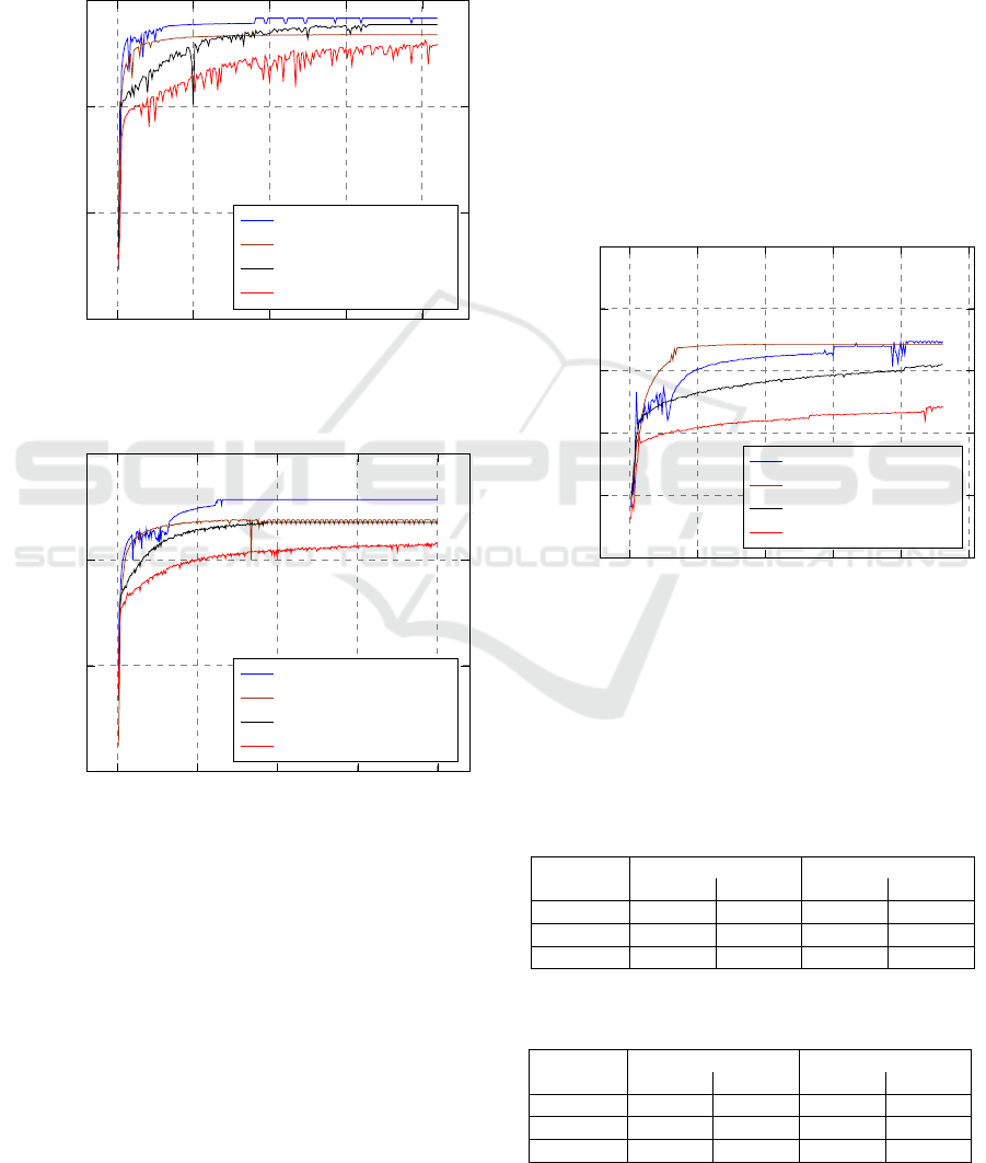
CNN this penalizes their overall performances. Ho-

wever, while on the experiments that have been per-

formed on Dataset 1 this gap in performance is not

that signiﬁcant, with the MLP and the CNN that still

obtain > 90% of accuracy, the same cannot be said for

the ones that have been run on Dataset 2 and Dataset

100

150

200

0.4

0.6

0.8

Epochs

Accuracy

MLP Bitmap Input

MLP Algebraic Input

CNN Bitmap Input

CNN Algebraic Input

Figure 1: The Testing Set accuracies on Dataset 1.

0 100 200 300 400

0.4

0.6

0.8

Epochs

Accuracy

MLP Bitmap Input

MLP Algebraic Input

CNN Bitmap Input

CNN Algebraic Input

Figure 2: The Testing Set accuracies on Dataset 2.

4.2 Dataset 2

On Dataset 2, a classiﬁcation task consisting of 15

classes, we observe in Figure 2 lower accuracies by

all the ANNs. But once more, the MLP trained with

the Bitmap Input is the ANN achieving the highest

accuracies. Besides this, we also observe that for the

CNNs, and in particular the one trained with the Alge-

braic Input, the increment in the amount of classes to

classify starts leading to worse results, which shows

the superiority of the MLPs. A superiority that beco-

mes evident on the experiments performed on Dataset

4.3 Dataset 3

This dataset corresponds to the hardest classiﬁcation

task on which we have tested the ANNs. As already

introduced, we have extended the Draw class with 6

different subclasses. As Figure 3 shows, the accura-

cies of all ANNs decrease due to the complexity of

the classiﬁcation task itself, but we see again that the

best performances have been obtained by the MLPs,

and in particular by the one trained with the Bitmap

Input. In this case, however, we observe that the lear-

ning curve is far more unstable when compared to the

one of the Algebraic Input. This may be solved with

more ﬁne tuning of the hyperparameters.

100

150

200

250

0.2

0.4

0.6

0.8

Epochs

Accuracy

MLP Bitmap Input

MLP Algebraic Input

CNN Bitmap Input

CNN Algebraic Input

Figure 3: The Testing Set accuracies on Dataset 3.

We summarize the performances of the ANNs on

the ﬁrst 3 datasets in the following tables. Table 1 re-

ports the accuracies obtained by the MLPs while Ta-

ble 2 shows the accuracies of the CNNs.

Table 1: The accuracies of the MLPs on the classiﬁcation

datasets.

Dataset

Bitmap Input Algebraic Input

ValSet TestSet ValSet TestSet

Dataset1 98.67% 96.07% 96.95% 93.58%

Dataset2 93.73% 93.41% 87.45% 87.28%

Dataset3 69.44% 68.33% 69.88% 66.21%

Table 2: The accuracies of the CNNs on the classiﬁcation

datasets.

Dataset

Bitmap Input Algebraic Input

ValSet TestSet ValSet TestSet

Dataset1 95.40% 95.15% 91.70% 90.33%

Dataset2 87.24% 87.10% 83.88% 83.72%

Dataset3 62.06% 61.97% 48.48% 46.86%

ICPRAM 2018 - 7th International Conference on Pattern Recognition Applications and Methods

280

With the regression experiment that aims to

train the ANNs to reproduce Stockﬁsh’s evaluation

function, we have obtained the most promising results

from all architectures. Table 3 reports the Mean Squa-

red Error (MSE) that has been obtained on the Valida-

tion and Testing Sets.

Table 3: The MSE of the ANNs on the regression experi-

ment.

ANN

Bitmap Input Algebraic Input

ValSet TestSet ValSet TestSet

MLP 0.0011 0.0016 0.0019 0.0021

CNN 0.0020 0.0022 0.0021 0.0022

We managed to train all the ANNs to have a Mean

Squared Error lower than 0.0025. By taking their

square root, it is possible to infer that the evaluations

given by the ANNs are on average less than 0.05 cp

off when compared to the original evaluation function

provided by the chess engine. Once again, the best

performance has been obtained by the MLP trained

on the Bitmap Input. The MSE obtained corresponds

to 0.0016, meaning that Stockﬁsh evaluates chess po-

sitions only ≈ 0.04 cp differently when compared to

our best ANN that does not use any lookahead. It is

also important to highlight the performances of the

CNNs. While during the classiﬁcation experiments

the superiority of the MLPs was evident, the gap bet-

ween CNNs and MLPs is not that large, even though

the best results have been obtained by the latter ar-

chitecture. Our results show in fact how both types

of ANNs can be powerful function approximators in

chess.

4.4 The Kaufman Test

In order to evaluate the ﬁnal performance of the

ANNs we have tested our best architecture with the

Kaufman Test

, a special dataset of 25 extremely com-

plicated positions, created by the back then Internatio-

nal Master Larry Kaufman (Kaufman, 1992). The test

has been speciﬁcally designed to evaluate the strength

of chess playing programs and has as main goal the

prediction of what, given a particular board state, is

considered as the best possible move. This optimal

move is chosen according to the evaluation that is gi-

ven by the strongest existing chess engines.

We have performed this experiment with the MLP

trained on the Bitmap Input on Dataset 4. The ANN

only evaluates the board states corresponding to a

lookahead depth of 1 node. This means that, given

The test can be downloaded in the PGN format from

http://utzingerk.com/test_kaufman

one particular position as input, it scores the possible

future board states corresponding to the set of candi-

date moves of depth 1, without exploring any further.

The ﬁnal move is the one corresponding to the highest

evaluation given by the ANN.

Besides checking if the move played by the ANN

corresponds to the one prescribed by the test we also

introduce the ∆cp measurement, which is able to esta-

blish the goodness or badness of the moves performed

by the ANN. We compute ∆cp as follows: we ﬁrstly

evaluate the board state that is obtained by playing

the move suggested by the test with Stockﬁsh. The

position is evaluated very deeply for more than one

minute, as a result we assign Stockﬁsh’s cp evalua-

tion to it. We name this evaluation δ

Test

. We then do

the same on the position obtained by the move of the

ANN in order to obtain δ

. ∆cp simply consists of

the difference between δ

Test

and δ

. The closer this

value is to 0, the closer the move played by the ANN

is to the one prescribed by the test.

Table 4 reports the results that have been obtained

on the Kaufman Test. For each position in the dataset

we show which is the best move that should be played

according to the test, and the move that has been cho-

sen by our ANN.

We observe that the MLP only plays Kaufman’s

optimal move twice, in Position 3 and in Position 6.

Even though at ﬁrst glance these results can seem di-

sappointing, a deeper analysis of the quality of the

moves played by the ANN lead to more promising re-

sults. Reconsidering the logic that has been used for

labeling positions as Draws in the classiﬁcation ex-

periments performed on Datasets 2 and 3, 17 moves

played by the ANN do not exceed a cp evaluation of

1.5. This means that, even though the move that is

chosen is not the optimal one, the position on the bo-

ard remains balanced. Furthermore, while the ANN

does not play the same move as the test dictates in

Position 1, this move was still evaluated equally well

by the engine. Hence a cp difference of 0.

There are, however, moves chosen by the ANN

that lead to a Losing position, in particular the ones

played in Positions 12, 14, 15, 19, 22 and 23. These

positions are very complex: they rely on deep look-

ahead calculations necessary to see tactical combina-

tions that are very hard to see, even for expert hu-

man players. Even though the ANN is still far from

the strongest human players it still reached an Elo ra-

ting of ≈ 2000 on a reputable chess server

. The

ANN played in total 30 games according to the follo-

wing time control: 15 starting minutes are given per

player at the start of the game, while an increment of

10 seconds is given to the player each time it makes a

https://chess24.com/en

Learning to Evaluate Chess Positions with Deep Neural Networks and Limited Lookahead

281

Table 4: Comparison between the best move of the Kauf-

man Test and the one played by the ANN. The value of 10

in position 22 is symbolic, since the ANN chose a move

leading to a forced mate.

Position Best Move ANN Move ∆cp

1 Qb3 Nf3 0

2 e6 Bd7 0.8

3 Nh6 Nh6 0

4 b4 Qc2 0.8

5 e5 e6 0.3

6 Bxc3 Bxc3 0

7 Re8 Bc4 0.1

8 d5 Qd2 0.9

9 Nd4 Ne7 0.3

10 a4 a3 0.1

11 d5 h5 1.2

12 Bxf7 Nf3 4.2

13 c5 Nxe4 1.7

14 Df6 f5 5.9

15 exf6 Bd4 4.6

16 d5 Rb8 0.6

17 d3 c4 0.8

18 d4 Qe1 1.4

19 Bxf6 h3 4.2

20 Bxe6 Bd2 1.7

21 Ndb5 Rb1 1.4

22 dxe6 Kxe6 10

23 Bxh7+ Nh4 5.7

24 Bb5+ b4 1.2

25 Nxc6 bxc6 0.6

move.

The ANN played against opponents with an Elo

rating between 1741 and 2140 and obtained a ﬁnal

game playing performance corresponding to a strong

Candidate Master titled player. The games show how

the ANN developed its own opening lines both when

playing as White and as Black and performed best du-

ring the endgame stages of the game, when the chan-

ces of facing heavy tactical positions on the board are

very small. The chess knowledge that it learned, al-

lowed it to easily win all the games that were played

against opponents with an Elo rating lower than 2000,

which correspond to ≈ 70% of the total games. Ho-

wever, this knowledge turned out to be not enough

to competitively play against Master titled players,

where only two Draws were obtained. An analysis

of the games shows how the chess Masters managed

to win most of the games already during the middle

game.

5 DISCUSSION

The results that have been obtained make it possible

to state three major claims. The ﬁrst one is related

to the superiority of MLPs over CNNs as best ANN

architecture in chess, while the second one shows the

importance of not providing the value of the pieces as

inputs to the ANNs.

We think that the superiority of MLPs over CNNs,

that is highlighted in our classiﬁcation experiments,

is related to the size of the board states. The large

success of CNNs is mainly due to their capabili-

ties to reduce the dimensionality of pictures while at

the same time enhancing their most relevant featu-

res. Chess, however, is only played on a 8 × 8 board,

which seems to be too small to fully make use of the

potential of this ANN architecture in a classiﬁcation

task. Generalization is made even harder due to the

position of the pieces. Most of the time they cover the

whole board and move according to different rules.

On the other hand, this small dimensionality is ideal

for MLPs since the size of the input is small enough to

fully connect all the features between each other and

train the ANN to identify important chess patterns.

Considering the importance of not providing the

ANNs with the material information of the pieces,

we have identiﬁed a bizarre behavior. Manual checks

show how the extra information provided by the Al-

gebraic Input is able to trick the ANNs especially in

endgame positions.

Last, but not least, considering the results obtai-

ned on the Kaufman Test and on the chess server, we

show that it is possible to create a chess program that

mostly does not have to rely on lookahead algorithms

in order to play chess at a high level. It is important to

mention however, that to make this possible, the ANN

needs to be able to learn as much domain knowledge

as possible. Taking inspiration from (Berliner, 1977),

we state that deep lookahead can be discarded as long

as it is properly compensated with relevant chess kno-

wledge.

Nevertheless, we are also aware that the perfor-

mance of the ANN still needs to be improved when it

faces heavy tactical positions. Hence, we believe that

the most promising approach for future work will be

to combine the evaluations given by the current ANN

together with quiescence search algorithms. By doing

so the ANN will be able to avoid the horizon effect

(Berliner, 1973) and also perform well on tactical po-

sitions.

6 CONCLUSION

We believe that this paper provides strong insights

about the use of ANNs in chess. Its main contributi-

ons can be summarized as follows: Firstly we propose

a novel training framework that aims to train ANNs to

ICPRAM 2018 - 7th International Conference on Pattern Recognition Applications and Methods

282

evaluate chess positions similar to how highly skilled

players do. Current State of the Art methods have al-

ways relied a lot on deep lookahead algorithms that

help chess programs to get as close as possible to an

optimal policy. Our method focuses a lot more on the

discovery of the pattern recognition knowledge that is

intrinsic in the chess positions without having to rely

on expensive explorations of future board states.

Secondly we show that MLPs are the most suit-

able ANN architecture when it comes to learning

chess. This is both true for the classiﬁcation expe-

riments as for the regression one. Furthermore, we

also show how providing the ANNs with information

representing the value of the pieces present on the bo-

ard is counter-productive.

To the best of our knowledge this is one of the few

papers besides (Oshri and Khandwala, 2016) that ex-

plores the potential of CNNs in chess. Even though

the best results have been achieved by the MLPs we

believe that the performance of both ANNs can be im-

proved. As future work we want to feed both ANN ar-

chitectures with more informative images about chess

positions and see if the gap between MLPs and CNNs

can be reduced. We believe that this strategy, appro-

priately combined with a quiescence or selective se-

arch algorithm, will allow the ANN to outperform the

strongest human players, without having to rely on

deep lookahead algorithms.

REFERENCES

Baxter, J., Tridgell, A., and Weaver, L. (2000). Learning to

play chess using temporal differences. Machine Lear-

ning, 40(3):243–263.

Berliner, H. J. (1973). Some necessary conditions for a mas-

ter chess program. In IJCAI, pages 77–85.

Berliner, H. J. (1977). Experiences in evaluation with BKG-

A program that plays Backgammon. In IJCAI, pages

428–433.

Chellapilla, K. and Fogel, D. B. (1999). Evolving neural

networks to play checkers without relying on expert

knowledge. IEEE Transactions on Neural Networks,

10(6):1382–1391.

David, O. E., Netanyahu, N. S., and Wolf, L. (2016). Deep-

chess: End-to-end deep neural network for automatic

learning in chess. In International Conference on Ar-

tiﬁcial Neural Networks, pages 88–96. Springer.

Fogel, D. B. and Chellapilla, K. (2002). Verifying Ana-

conda’s expert rating by competing against Chinook:

experiments in co-evolving a neural checkers player.

Neurocomputing, 42(1):69–86.

Kaufman, L. (1992). Rate your own computer. Computer

Chess Reports, 3(1):17–19.

Krizhevsky, A., Sutskever, I., and Hinton, G. E. (2012).

Imagenet classiﬁcation with deep convolutional neu-

ral networks. In Advances in neural information pro-

cessing systems, pages 1097–1105.

Lai, M. (2015). Giraffe: Using deep reinforcement learning

to play chess. arXiv preprint arXiv:1509.01549.

Oshri, B. and Khandwala, N. (2016). Predicting moves in

chess using convolutional neural networks. Stanford

University Course Project Reports-CS231n.

Patist, J. P. and Wiering, M. (2004). Learning to play draug-

hts using temporal difference learning with neural net-

works and databases. In Benelearn’04: Proceedings

of the Thirteenth Belgian-Dutch Conference on Ma-

chine Learning, pages 87–94.

Romstad, T., Costalba, M., Kiiski, J., Yang, D., Spitaleri,

S., and Ablett, J. (2011). Stockﬁsh, open source chess

engine.

Schaul, T. and Schmidhuber, J. (2009). Scalable neural net-

works for board games. Artiﬁcial Neural Networks–

ICANN 2009, pages 1005–1014.

Sifaoui, A., Abdelkrim, A., and Benrejeb, M. (2008). On

the use of neural network as a universal approximator.

International Journal of Sciences and Techniques of

Automatic control & computer engineering, 2(1):336–

399.

Silver, D., Huang, A., Maddison, C. J., Guez, A., Sifre,

L., Van Den Driessche, G., Schrittwieser, J., Antonog-

lou, I., Panneershelvam, V., Lanctot, M., et al. (2016).

Mastering the game of Go with deep neural networks

and tree search. Nature, 529(7587):484–489.

Sutton, R. S. (1988). Learning to predict by the methods of

temporal differences. Machine learning, 3(1):9–44.

Sutton, R. S. and Barto, A. G. (1998). Reinforcement le-

arning: An introduction, volume 1. MIT press Cam-

bridge.

Tesauro, G. (1994). TD-gammon, a self-teaching back-

gammon program, achieves master-level play. Neural

computation, 6(2):215–219.

Thrun, S. (1995). Learning to play the game of chess. In

Advances in neural information processing systems,

pages 1069–1076.

van den Dries, S. and Wiering, M. A. (2012). Neural-

ﬁtted td-leaf learning for playing othello with struc-

tured neural networks. IEEE Transactions on Neural

Networks and Learning Systems, 23(11):1701–1713.

van den Herik, H. J., Donkers, H., and Spronck, P. H.

(2005). Opponent modelling and commercial games.

In Proceedings of the IEEE 2005 Symposium on Com-

putational Intelligence and Games (CIG’05), pages

15–25.

Learning to Evaluate Chess Positions with Deep Neural Networks and Limited Lookahead

283