Computer Vision based System for Apple Detection in Crops

Mercedes Marzoa Tanco, Gonzalo Tejera and J. Mat

ıas Di Martino

Facultad de Ingenier

ıa, Universidad de la Rep

ublica, J. Herrera y Reissig 565, Montevideo, Uruguay

Keywords:

Apple Detection, Image Processing, Fruit Recognition.

Abstract:

In recent times there has been an increasing need to improve apple production competitiveness. The automatic

estimation of the crop yield or the automatic collection may contribute to this improvement. This article

proposes a simple and efﬁcient approach to automatically detect the apples present on a given set of images.

We tested the proposed algorithm on several images taken on many different apple crops under natural lighting

conditions. The proposed method has two main steps. First we implement a classiﬁcation step in which each

pixel is classiﬁed as part of an apple (positive pixel) or as part of the background (negative pixel). Then, a

second step explore the morphology of the set of positive pixels, to detect the most likely conﬁguration of

circular structures. We compare the performance of methods such as: Support Vector Machine, k-Nearest

Neighbor and a basic Decision Tree on the classiﬁcation step. A database with 266 high resolution images

was created and made publicly available. This database was manually labeled and we provide for each image,

a label (positive or negative) for each pixel, plus the location of the center of each apple.

1 INTRODUCTION

Currently there is an increasing need to obtain higher

quality products at a lesser cost, thus increasing com-

petitiveness. Developing automatic systems to enable

the use of human resources more efﬁciently in terms

of precision, repeatability or time consumed is a good

alternative. Also, estimating crops yield helps pro-

ducers improve the quality of their fruit and reduce

operation costs. Managers can use estimation results

to plan the optimal capacity for packaging and storage

(Robinson, 2006). As an example, the cost of harves-

ting citrus fully by hand may range from 25% to 33%

of the total cost of production (Dougherty and Lotufo,

2003).

The overall objective of this article is to intro-

duce an automated computer vision system for the de-

tection and counting of red apples in trees. The pre-

sent work is part of the design of a more complex sy-

stem for the automatic estimation of crops yield and

harvesting.

In order to detect pixels belonging to apples, three

techniques are evaluated: Support Vector Machines

(SVM), K-Nearest Neighbors (k-NN) and a very sim-

ple decision tree (DT). As an improvement to the out-

come of pixel detection, morphology operations have

been used. In order to detect the apples themselves,

and given their shape, the Hough transform for circles

has been used. Finally, a post-processing of the circles

found is made, to rule out false positives detections.

2 RELATED WORK

There are several works on the detection of fruit using

computer vision techniques.

There are two great approaches to the estima-

tion of a crop yield, one is counting the apples and

the other is doing the estimation through ﬂower den-

sity. Several researchers have worked in the ﬁrst cate-

gory using color images (Linker et al., 2012),(Rakun

et al., 2011),(Tabb et al., 2006), hyperspectral ima-

ging (Safren et al., 2007), and thermal imaging (Sta-

jnko et al., 2004). Aggelopoulou et al. (Aggelopoulou

et al., 2011) worked on the second category, sampled

images of trees in an apple orchard and found a cor-

relation between ﬂower density and crop yield. Ho-

wever, this method encounters a problem: the period

between the ﬂowering and the crop is too long and

there are multiple unpredictable factors, such as we-

ather conditions, which make the correlation exposed

to variations from one year to the next.

Counting apples using computer vision puts for-

ward several challenges, the most important of which

being the variation of natural light, the occlusion of

fruits due to foliage, branches and other fruits and the

Tanco, M., Tejera, G. and Martino, M.

Computer Vision based System for Apple Detection in Crops.

DOI: 10.5220/0006535002390249

In Proceedings of the 13th International Joint Conference on Computer Vision, Imaging and Computer Graphics Theory and Applications (VISIGRAPP 2018) - Volume 4: VISAPP, pages

239-249

ISBN: 978-989-758-290-5

239

detection of one same apple in several images. Follo-

wing are the techniques used by different authors to

elude these challenges.

Wang et al. (Wang et al., 2013) present one way

to avoid the variation of light by acquiring images at

night with artiﬁcial illumination. The solution given

by Jimenez et al. (Jim

enez et al., 1999) to the occlu-

sion is a post-processing of the images using Hough

transforms with ellipses. Finally, for the challenge of

multiple detections of the same apple in a sequence

of images, Wang et al. (Wang et al., 2013) propose

the use of a pair of stereo cameras to estimate the po-

sition of the apples and rule out those that coincide.

A computer vision algorithm detects and registers ap-

ples that appear in sequential images and then counts

them for the estimation. They had good results both

in red and green apples and they make a full study

of cases with results according to the type of cut of

the trees, quantity of spots in the apples, accumula-

tion of apples and occluded environments. Speciﬁ-

cally, they carry out the identiﬁcation of red apples by

the following stages: through a hue threshold (H) and

a saturation threshold (S), the pixels complying with

the apples characteristics are detected and then, the

apples are segmented individually using morphology

operations. Finally, they look for the global position

of the apple, thus avoiding to count it more than once.

Gongal et al. (Gongal et al., 2016a) proposed a si-

milar approach, were in addition to a pair of stereo

images, a tunnel structure has build to minimize na-

tural illumination effect which enable to reduced the

variability in lighting condition. Images captured in a

tall spindle orchard were processed. Zhao et al. (Zhao

et al., 2005) present a method to identify apples using

a single RGB image under natural illumination as in-

put. To that end, they ﬁrst deﬁne a redness measure

as r = 3R − (G + B), where R, G and B represent the

red, green and blue values respectively of each pixel,

then they apply morphological operations and ﬁnally

an edge detection ﬁnal step. Ji et al. (Ji et al., 2012)

use the same kind of input RGB images as the previ-

ous work, and apply a median ﬁlter to eliminate the

noise followed by a classiﬁcation step in which they

use SVM algorithm on a color plus shape space. Ji-

menez et al. (Jim

enez et al., 1999) propose an auto-

matic fruit recognition system and present a schema-

tic review of the works developed until the end of the

nineties. Their fruit detection methodology is able to

recognize spherical fruits in natural conditions using

a laser range ﬁnder which provide range/attenuation

data of the sensed surfaces. Their recognition system

uses a laser range ﬁnder model and a dual color/shape

analysis algorithm to locate the fruits.

The work presented by Wang et al. (Wang et al.,

2013) is likely the closest work to the present arti-

cle. However, signiﬁcant differences exist between

this work and the present article. In ﬁrst place Wang

et al. propose a system that uses a two-camera ste-

reo rig for image acquisition and works at nighttime

with controlled artiﬁcial lighting to reduce the vari-

ance of natural illumination. While we work in am-

bient uncontrolled illumination conditions and use a

single RGB camera. In addition, from the point of

view of the numerical methods presented, we extend

Wang et al. approach by including more advanced

machine learning techniques and by facing apple de-

tection problem in the context of an imbalanced pro-

blem (Barandela et al., 2003; Japkowicz and Stephen,

2002; Liu et al., 2009).

The main contributions of the present work are:

(i) We improve previous approaches by the use of

more robust machine learning techniques. In parti-

cular, by facing the pixels classiﬁcation problem as a

pattern recognition imbalanced problem. (ii) We pre-

sent an updated review of the current state of the art.

(iii) A database with 266 high resolution images was

created and made publicly available (Marzoa, 2017a)

.This database was manually labeled and we provide

for each image, a label (positive or negative) for each

pixel, plus the location of the center of each apple. To

the best of our knowledge is the ﬁrst publicly availa-

ble database with such characteristics.

3 PROPOSED SOLUTION

This section describe the methods used to solve the

problem posed. The methodology applied can be se-

parated in three stages: construction of the database,

classiﬁcation of the pixels in apple or background and

identiﬁcation of the apples themselves.

3.1 Construction of the Database

The database is formed by 266 images acquired using

natural light, at “Las Brujas - INIA” experimental sta-

tion located in Canelones, Uruguay. Each image has

an associated binary image where it is indicated, in

white, whether the pixel belongs to an apple, or in

black, if not. In its turn, there is a ﬁle per image with

the coordinates of each apple’s center. The data base

is available for future works (Marzoa, 2017a).

3.2 Classiﬁcation of Pixels in Apple or

Background

To classify the apple pixels, a classic pattern recogni-

tion pipeline was followed. First a set of discrimina-

VISAPP 2018 - International Conference on Computer Vision Theory and Applications

240

tive features is proposed to map the input RGB pixels

to a more suitable feature space. Then, different clas-

siﬁers are trained and evaluated.

3.2.1 Feature Extraction

To describe those pixels that belong to an apple and

those that belong to the background we use three ba-

sic features: Hue (H), Saturation (S), and a simple

Texture descriptor.

Hue and Saturation. Apples have a reddish tonality

which is different from almost all the other objects

in a crop; therefore, tonality is a good differentiating

characteristic.

In order to have robust representation of pixels un-

der different illumination conditions, the input color

space RGB is mapped into the HSV (Hue, Satura-

tion, and Value) color space (Manjunath et al., 2001).

The Hue and Saturation values are directly related to

the color perceived of the pixels, while the Value is

mainly related to the lightness of the scene.

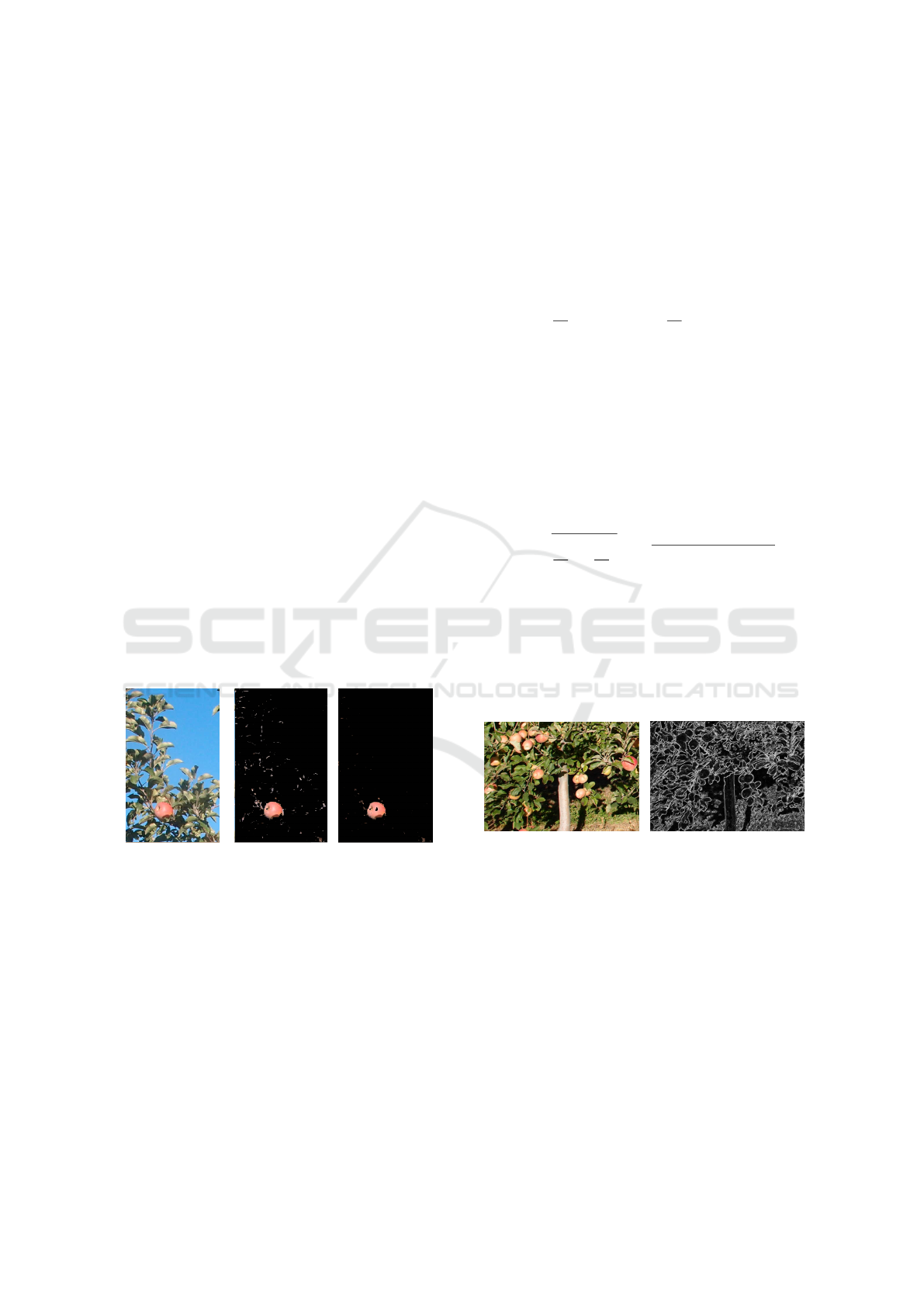
The ranges of values of H with which better re-

sults are obtained were determined for each techni-

que used. Tonality H is not deﬁned for white, gray

or black, that is why saturation, has to be used to ex-

clude them. Figure 1(a) illustrates a test image of the

database, Figure 1(b) show the result of segmenting

the test image according to its values of H and Figure

1(c) show the result of segmenting using both H and

(a) Input image (b) After Hue

segmentation

and Saturation

segmentation

Figure 1: Example of segmenting a test image using diffe-

rent features.

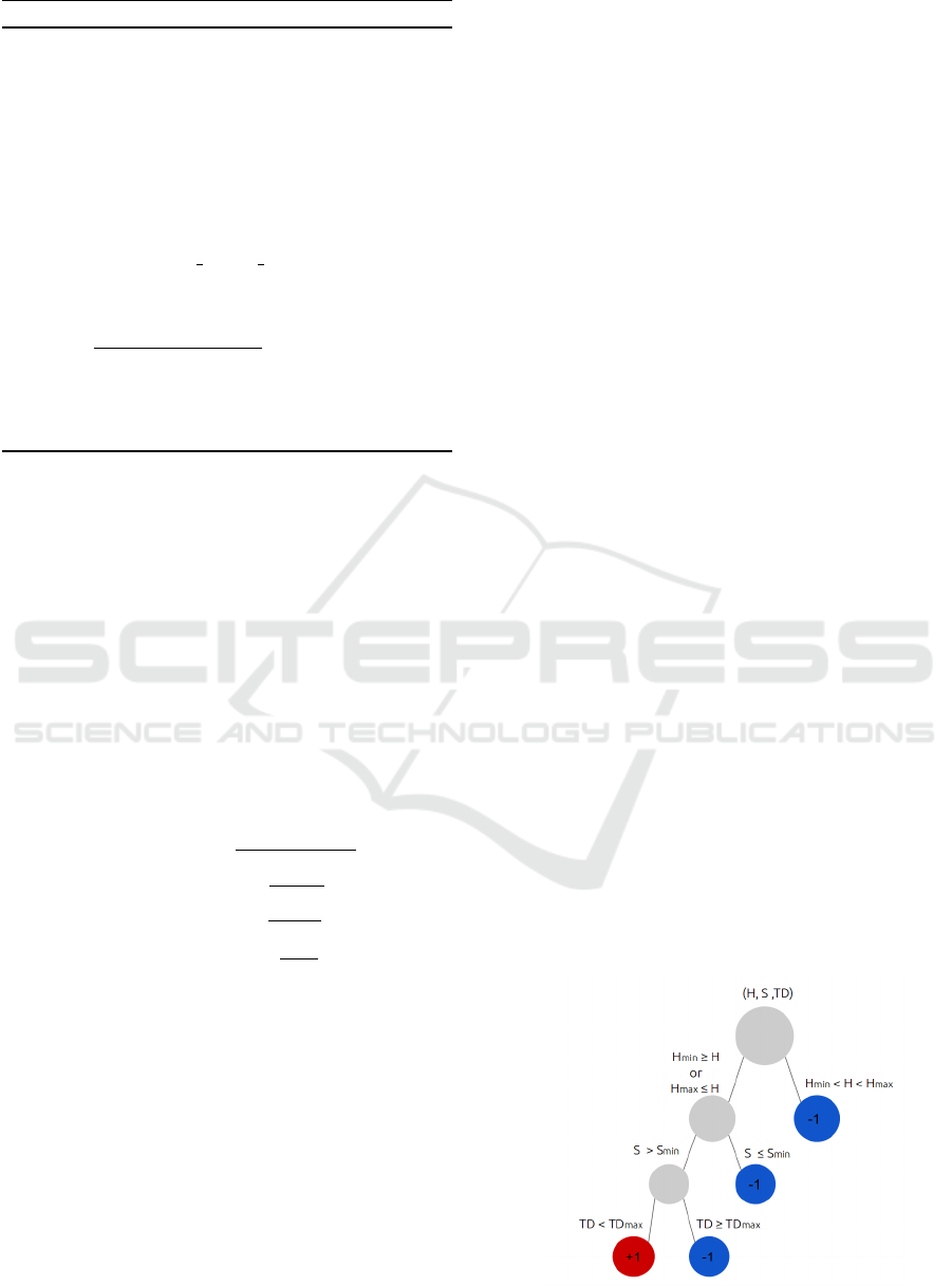
Texture Descriptor. Another visible characteristic is

that apples have less edges in their surface than grass,

leaves or trunks. An edge may be seen as the place

where the intensity of pixels changes dramatically (or

noticeably), and this is obtained through partial deri-

vatives. A large change in a gradient means a large

change in the image. A method to detect edges in an

image is then to place the pixels where the gradient is

larger than the neighbors or, to generalize, where it is

larger than a certain threshold.

In the present work, the Sobel operator (Szeliski,

2010) is used to estimate the gradient of the intensity

for a given image. For each pixel, the operator gives

the magnitude and the direction of the larger possible

change.

Mathematically, two square n ×n kernels are deﬁ-

ned, G

and G

. Then, the continuous spatial deriva-

tives are numerically approximated as,

∂I

∂x

≈ G

∗ I and

∂I

∂y

≈ G

∗ I (1)

where ∗ denotes the two dimensional convolution

operation.

Kernels G

and G

are deﬁned as,





1 0 1

−2 0 2

−1 0 1





, G





1 −2 −1

0 0 0

1 2 1





(2)

For each pixel of the image, an approximation of

the gradient at the said point is estimated as,

|∇I| =

∂I

∂x

∂I

∂y

∗ I)

+ (G

∗ I)

. (3)

Finally, edges can be deﬁned as the set of pixels

{x : |∇I(x)| > τ} for a given threshold τ. By represen-

ting the edges with pixels in white, in ﬁgure 2 the ef-

fect of applying Sobel ﬁlter to an image may be seen.

Speciﬁcally, it may be observed how, while apples ba-

rely exhibit edges in their surface, leaves and the grass

do.

(a) Input image (b) Edgedes after aplying

Sobel

Figure 2: Example of image after apply Sobel.

Algorithm 1 summarizes the main steps of the fe-

ature representation step.

Notation. The features space deﬁned for this pro-

blem is a three dimensional space where each pixel

sample will be represented by a feature vector x =

(h,s,td)

∈ R

, h and s correspond to the featu-

res associated to the hue and saturation respectively,

while td denotes the “texture descriptor” obtained

from image’s gradient. Those pixels label as belon-

ging to an apple, will be refer as positive while pixels

associated to the background will be refer as negative.

Numerical label 1 and −1 will be associated to

Computer Vision based System for Apple Detection in Crops

241

Algorithm 1: Features of an image.

Input : RGB image I : H ×W × 3 matrix

Output: 3D matrix X : H ×W × 3 // Hue,

Saturation, and Texture

Descriptor for each pixel.

// Map RGB space to HSV space

1 I

HSV

= rgb2hsv(I)

2 X(:,:,1) = I

HSV

(:,:,1)

3 X(:,:,2) = I

HSV

(:,:, 2)

// Define Sobel kernels (2)

4 (G

) = define sobel kernels()

// Convert RGB to a gray image

5 I ← rgb2gray(I) // Compute im.

gradient modulus

6 I ←

(I ∗ G

)

+ (I ∗G

)

// Local gradient descriptor

7 X(:,:,3) = I

8 return X

positive and negative classes respectively. A true po-

sitive/negative pixel will be a positive/negative pixel

correctly classiﬁed, while a false positive/negative re-

sult will be a negative/positive sample misclassiﬁed.

3.2.2 Performance Measurement

Let us recall some well known performance measu-

rements widely applied in the context of imbalanced

problems (Di Martino et al., 2012; Di Martino et al.,

2013b; Di Martino et al., 2013a; Kubat et al., 1997;

Barandela et al., 2003; Garc

ıa et al., 2012). Given

T P, T N, FP and FN as the number of true posi-

tive, true negative, false positive and false negative

respectively, we deﬁne,

Accuracy: A =

T P+T N

T P+T N+FP+FN

(4)

Recall: R =

T P

T P+FN

(5)

Precision: P =

T P

T P+FP

(6)

F-measure: F

R P

P +R

(7)

Accuracy (or equivalently the error rate) is one of

the most popular measures used to deﬁne optimality

in pattern recognition problems. However in the con-

text of highly imbalanced problems is not an adequate

way of measuring and comparing different strategies

performance. Let illustrate this point with a simple

example. If just the 1% of the pixels of a set of images

corresponds to pixels that belongs to an apple, we can

design a trivial algorithm that classiﬁes all the pixels

as part of the background, i.e. the output label of this

method is always −1. This approach will achieve an

accuracy of 99% while non a single pixel nor a single

apple will be detected. Precision and Recall are two

important measures to evaluate the performance of a

given classiﬁer in an imbalance scenario. The Recall

indicates the True Positive Rate, while the Precision

indicates the Positive Predictive Value. It is clear that

improving the recall will impact on the precision and

vice-versa, so it is important to combine them in a sin-

gle measurements, which is obtained by considering

the F-measure.

3.2.3 Classiﬁers

Following is a description of the techniques evalua-

ted for the classiﬁcation of images pixels. We tes-

ted three different algorithms: a very simple decision

tree, K-Nearest Neighbor and Support Vector Ma-

chine(Bishop, 2006). The ﬁrst technique is extremely

simple and efﬁcient, and is likely the strategy that one

must follow if the hardware resources are very limi-

ted. The other two methods are more advanced ma-

chine learning algorithms that for similar applications

showed robust results in the past.

Decision Tree. A decision tree enables to classify a

pattern in different classes. The tree nodes represent

the questions of a certain property; the branches, the

possible values of a property and each node leave re-

presents one category. The pattern tested is allotted

to the category attained. The links are mutually ex-

cluding and exhaustive. The main reasons to include

such a simple technique are: ﬁrstly, to see how ex-

tremely simple strategies work in order to evaluate if

the complexity of more sophisticated machine lear-

ning algorithms is justiﬁed. And secondly, to have

very simple and efﬁcient solution that can be embed-

ded in robot prototypes with very limited hardware

resources. With this ideas in mind, we propose the

use of a simple tree structure with three nodes and

four leafs, as it illustrated in Figure 3. This method

has four free parameters that need to be tune: H

min

max

, S

min

and T D

max

. To that end, a training data-

set and an optimality criteria needs to be set. In the

experimental section this aspects will be addressed.

Figure 3: Scheme of the simple tree structure evaluated.

VISAPP 2018 - International Conference on Computer Vision Theory and Applications

242

K-Nearest Neighbor (KNN). Once the features are

deﬁned and the data is mapped to this feature space,

it is to be expected that pixels of the same class will

be close with respect to each other on this domain.

This is the basic idea behind the KNN technique. This

technique consists of classifying the incoming point

starting from its spacial location in the dominion of

features, and to classify it in function of its nearest

neighbors.

Choosing a right value of K is critical in KNN,

since, if too small a K is taken, we would often en-

counter mistaken classiﬁcations for those pixels that

are in the limit between two classes, while if a very

large K is taken, the cost of looking into all the neig-

hbors is too big and the class boundaries on the feature

space may be blurred.

Support Vector Machine (SVM). Given a set of trai-

ning examples where the data are marked as belon-

ging to one class or the other, the training algorithm

SVM builds a model to adjust each of the classes. By

intuition, SVM constructs a model representing the

training points in the space, separating the classes by

the widest margin possible. When the new examples

are put in correspondence with the said model, they

are classiﬁed in one class or the other according to

what side of the gap they are (Hearst et al., 1998).

These types of algorithms seek the hyperplane

with the greatest distance, or margin, with the points

nearest it itself. In this way, the points of the vector

labeled with one category will be on one side of the

hyperplane and the cases that are in the other category

will be on the other side.

The representation through kernel functions

(Scholkopf and Smola, 2001) offers a solution to the

problems in which the classes are not linearly sepa-

rable, by projecting the data into a space of greater

dimension.

In this work a Gaussian radial basis kernel

function (Scholkopf and Smola, 2001) is used,

) = e

−

− x

2σ

(8)

This classiﬁer has in total two free parameters that

need to be set: σ which determines the shape of the

kernel, and ν that set the compromise between the va-

lue of the margin and the amount of errors on SVM

optimization (Hearst et al., 1998).

3.2.4 Implementation Details

The code is written in c++. To implement SVM,

the functions given by OpenCV (OpenCV, 2017) are

used. To implement KNN, the functions given by

OpenCV to interface the FLANN (Muja and Lowe,

2009) library are used.

3.3 Counting of Apples

After having classiﬁed the pixels of an input image as

part of an apple or the background, we have a groups

of pixels labeled as apples, not their quantity or lo-

cation. The next step was then to identify the apples

within those groups of pixels. In order to do that, we

resorted techniques applied to a binary image where

the background is set as black and pixels that belong

to an apple are set as white. The process we applied

consists of the following three stages: (i) Pixels Mask

Pre-processing, (ii) Detection of circles, and (iii) Cir-

cles Validation.

Pixels Mask Pre-processing. First applied mor-

phological operations to remove the noise and to

smoothen the regions edges. This helped to detect ci-

rcles and rule out regions with a small area.

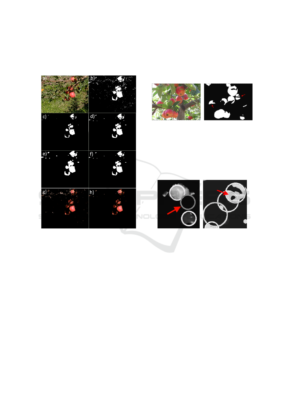
In the result of the recognition of apple pixels,

there are regions with areas of diverse sizes, from re-

gions of signiﬁcant size to others that are nothing but

a small set of noise pixels as seen in ﬁgure 4. The

noise is generated by the foliage, branches and other

elements that, due to their features resemble those of

the apples, but that are actually isolated small regions

that should be ruled out.

(a) Input image (b) After clasiﬁcation of

pixels

Figure 4: Recognition of apple and background pixels be-

fore process the mask pre-processing.

The use of the morphological operations erosion

and dilation is proposed. Erosion leads to the removal

of the noise and the reduction of small regions, but it

also leads to an increase in the gaps contained in the

regions of signiﬁcant size. On the other side, the di-

lation generates the opposite phenomenon, expansion

of the regions and reduction of the gaps within them.

For this reason four stages of morphological operati-

ons were applied, as seen in ﬁgure 5. At a ﬁrst stage,

the aim is to remove the noise without modifying the

size of the area of the signiﬁcant size regions and, at a

later stage, the aim is to smoothen the edges and join

the adjacent regions, keeping also approximately the

original size of each area.

As structuring element, a circle is used, due to its

proximity to the shape in which the apples appear in

the images. The size of the circle must be set in order

Computer Vision based System for Apple Detection in Crops

243

to remove the noise but taking care not to remove re-

gions of interest. In the following section there is an

evaluation of the more adequate size starting from the

experiments results.

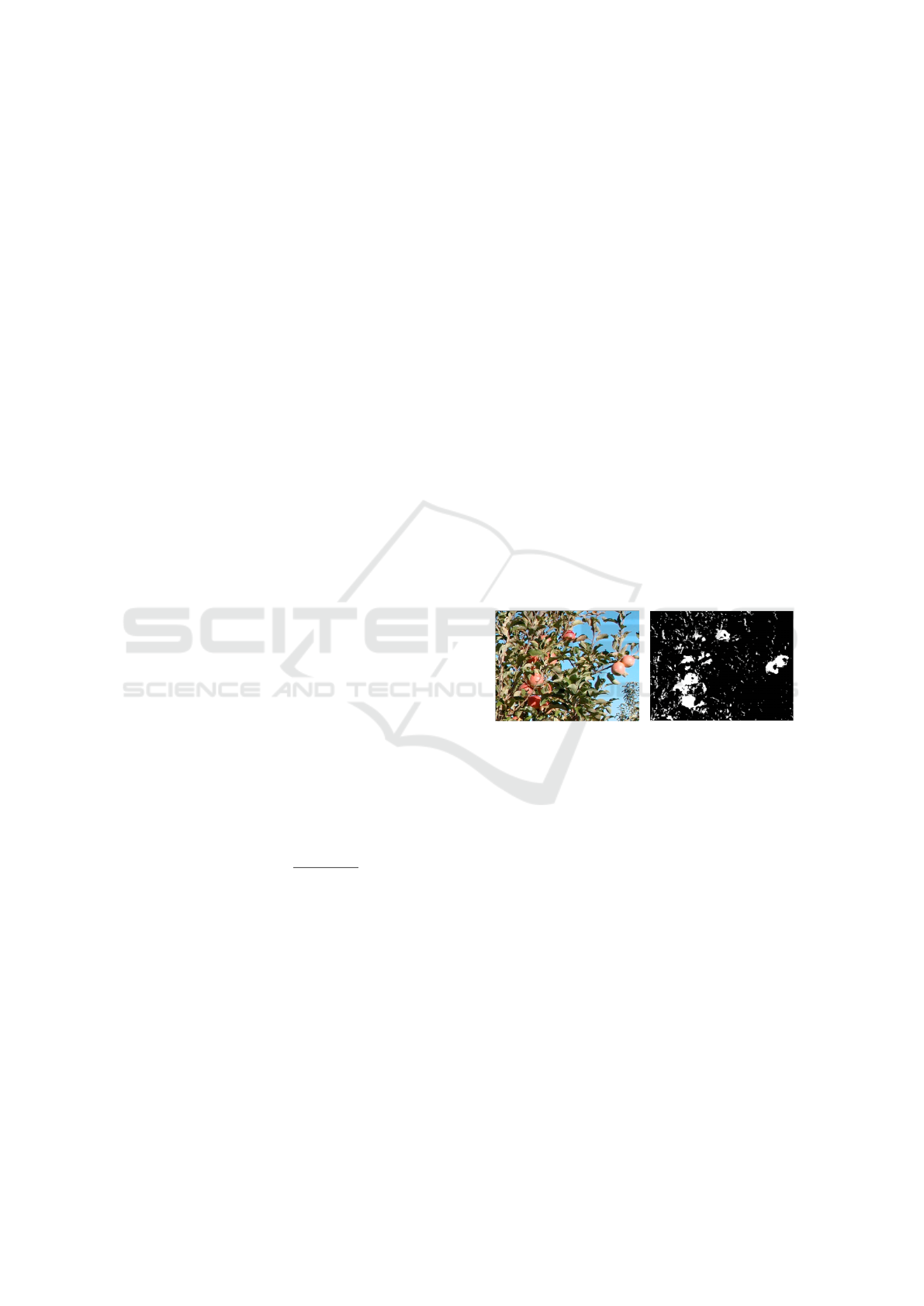
Figure 5: Stages of morphological operations (a) Original

Image (b)Mask of pixel classiﬁcation (c)Erosion (d) Dilata-

tion (e) Dilatation (f) Erosion (g) RGB Mask of pixel clas-

siﬁcation (h) RGB Mask after applying morphological ope-

rations.

Detection of Circles. At a second stage, we recog-

nize the circles present in the binary image which is

the result of the recognition of the pixels. Since ap-

ples present a geometrical shape very near a sphere,

in two dimensions images they will be seen as circles,

whatever the location where the image is acquired.

The Hough transform for circles (Brunelli, 2009)

is used as method to recognize the circles present in

the binary images obtained after the previous step.

Cicles Validation. The last stage, after having obtai-

ned a collection of circles with their radius and cen-

ters, consists of studying each one of them in order to

validate which of the candidate circles actually repre-

sent an apple in the ﬁgure. Too occluded apples will

generate small areas but not so much as to be ruled out

by the morphological operations. If, moreover, they

exhibit curved edges, a circle will be detected which,

while belonging to an apple, does not represent that

apples real location. Also, it may well be that, by

being occluded, one same apple may generate more

than one separated and curved area, thus resulting in

only one apple being counted as several. Examples of

the previous situations are illustrated in Figure 6.

(a) Input image (b) Mask after pixel classiﬁ-

cation

Figure 6: Example of how an apple may generate more than

one separated area or a curved are.

Another possible situation may be seen in Fi-

gure 7(a). In this case a circle was detected because

the higher region presents an outward circular curve,

which leads to the detection of indicated circle. As a

result, an empty circle is detected inside it.

(a) (b)

Figure 7: Wrong circles detected because the higher region

presents an outward circular curve or because a region exhi-

bits circular gaps inside.

To avoid detecting wrong circles, we suggest ru-

ling out detected circles whose area is less than a mi-

nimum area. This means that, for each circle, the area

of the region it includes is studied and the circle will

be ruled out if the said area is less than a deﬁned per-

centage of the total are of the circle.

The second stage within the post-processing of ci-

rcles is to study the intersection of the circles.

As seen in ﬁgure 7(b), if a region exhibits circular

gaps inside it is possible that more than a circle will be

detected in it. To avoid these false detections, the area

in each circle is studied and the region that intersects

with other circles already studied is deducted.

In the case of ﬁgure 7(a), where ﬁrst the higher ci-

rcle is detected, we study the area of the second circle

and deduct the intersection marked with the red arrow.

In this case, the second circle will be ruled out, since

VISAPP 2018 - International Conference on Computer Vision Theory and Applications

244

the area is too small. If, on the contrary, the remaining

area of the second circle is noticeable, it would not be

ruled out but would be taken as a second apple.

Algorithm 2 summarizes the main steps perfor-

med for the detection of apples on the binary mask

obtained after the pixel classiﬁcation.

Algorithm 2: Apple detection.

Input : Mask result of pixels classiﬁcation

M : H ×W × 1

Output: List of centers and radiuses of the

circles circles ok

// Morphological operations

1 M = erode(M) // Eliminates noise

2 M = dilate(M)

3 M = erode(M) // Smooths regions

4 M = dilate(M)

// Find circles

5 circles(1,:) = HoughCircles(M)

6 circles ok = NULL

7 for each c in circles do

// Discard circles whose area is

less than a minimum area

8 mask c = new image()

9 mask c =

circle(mask c,c.center, c.radius)

mask = mask c & M

p = countNonZero(mask) ∗

100/(c.radius

∗ π)

10 if p > area ok then

// Study the region that

intersects with other

circles already studied

11 intersected circles =

intersected circles(c,circles ok)

12 if intersected circles is NULL then

13 circles ok.add(c)

14 else

15 mask intersec = mask c

16 for each c int in

intersected circles do

17 mask intersec =

mask intersec − c int

19 p =

countNonZero(mask intersec) ∗

100/(c.radius

∗ π)

20 if p > area intersect ok then

21 circles ok.add(c)

22 return circles ok

4 TRAINING STEP

This section present the results obtained in the trai-

ning step, considered according to each technique stu-

died and their comparison. Cross validation with 10

iterations is used for all trainings.

4.1 Data Base

In classiﬁcation works using computer vision, the da-

tabase is an essential cornerstone; it is from this that

the condition of effectiveness of the techniques stu-

died are set. In this case the database is composed

by images acquired in the outdoor, with natural light,

seeking variety in them in order to be as close to re-

ality as possible. The database created besides the

images includes a labeling of which pixels belong to

apples and which to background, as well as the coor-

dinates of the center of each apple.

Since the database has 266 images, with an

average resolution of 600x800, there is an approxi-

mate total of 63.840.000 pixels, which requires a me-

mory structure of almost 64 million places, and this

has to be multiplied by three, since the features being

evaluated are three. It is then of utmost importance to

carry out a study of the minimum percentage of pixels

required that will be taken, so that it can be an accep-

table representation of the total of the pixels in the da-

tabase. In view of this, the percentage is changed and

the pixels are classiﬁed (as apple or non apple) using

the decision tree, given that this is the technique that

requires less execution time. By increasing the quan-

tity of pixels, after using 0.4% of the total of pixels,

the measure of success used (f-measure) remains sta-

tionary.

4.2 Fitting for the Parameters of Apple

Pixels Detection

Following is the ﬁtting of the parameters for each

technique.

Decision Tree. The valid values for the parameters

studied are as follows: Hue in a range between 0 and

180, Saturation between 0 and 255 and edge density

between 0 and 100.

The values that gave the best results for the deci-

sion tree were: Min H = 13, Max H = 161, Min S =

47 and max edges = 76.

K Nearest Neighbor. Due to the features of the KNN

method when in a problem of imbalanced classes, it

is necessary to limit the percentage for the training of

the biggest class. In its turn, the quantity of nearest

neighbors considered, K, should be determined.

Computer Vision based System for Apple Detection in Crops

245

Support Vector Machine. The study of effective-

ness and efﬁciency was made by varying parame-

ters gamma and C of the kernel, gamma being the

weight of each points inﬂuence while C exchanges

wrong classiﬁcation against surface simplicity. The

values that returned best results being C = 100 and

gamma = 1.

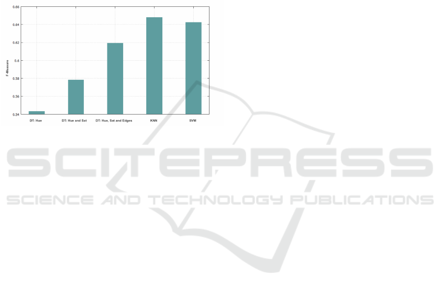
Comparison of Techniques. Comparing the results

obtained by using the three techniques, we have that

KNN is the technique that yields the best results, as

seen in ﬁgure 8. Also, it shows the improvement bet-

ween using only one characteristic and using three.

Figure 8: F-measure average obtained in the recognition of

apple pixels. First it shows the improvement of using three

characteristics with tree decision and then the comparison

using KNN and SVM.

Since the three techniques used the same domi-

nion of characteristics for their classiﬁcation, it is in-

teresting to compare the classiﬁcation of each of the

methods for a set of points normalized from 0 to 1 (a

cube) of the three characteristics; they may be seen in

3D, as shown in ﬁgure 9.

It is observed how, while the cloud of apple pixels

is similar in the three methods, KNN and SVM do not

present straight borders, which is closer to reality.

Morphology. The study of the morphology parame-

ters was made using the Decision Tree technique be-

cause is more quickly that the others. The parameters

used for the technique are who gives better results of

f-measure. It was used cross validation, using values

between 1 and 10 for the radios, obtaining the bests

results when use radio of 5px for erode and 7px for

dilation.

4.3 Fitting for the Parameters of Apples

Detection

Following is the ﬁtting of parameters for the detection

of the apples in themselves. First there is a description

of the parameters used to detect the Hough circles and

then of the parameters used for the post-processing.

Detection of Hough Circles. The minimum distance

between circles detected and the accumulator thres-

hold was varied. The minimum and maximum radium

was determined by estimating the average radius in

the database: the values were 20 and 75 pixels, re-

spectively.

In order to ﬁnd out whether the circle found is the

same one labeled at the database only by using their

centers, in most cases they would be found not to coi-

ncide, so a margin of tolerance between centers equal

to the value of the radius of the circle found is used.

The Hough transform uses two values to be de-

termined: the minimum acceptable distance among

circles and an accumulator that indicates the percen-

tage that should coincide in the image with the circle

found. The values obtained for the detection of cir-

cles that gives better, with an average distance among

circles of 67 and an accumulator of 8.

Post-processing in Circles. Using 20% of the area of

an apple as minimum area for a circle to be considered

valid, better results are obtained by giving an average

FV of 0,53 ± 0, 04.

In the table 1 it shows the values of all the para-

meters used in the project.

5 RESULTS

The proposed approach for automatic apple detection

consists on two main steps as was described in the

previous Sections. Firstly, the individual pixels of

each input image are classiﬁed as Positive or Negative

(recall that the positive class is associated to pixels

that potentially belong to an apple). Secondly, the

morphology of the set of Positive pixels is analyzed

to ﬁnd circular structures that lead to the ﬁnal goal

of detecting the apples present in the target image. It

is clear that the individual performance of both sta-

ges will impact on the overall performance of the pro-

posed approach, and so both steps need to be care-

fully analyzed and trained as explained in the previ-

ous Section.

Let us start by analyzing the results obtained for

the classiﬁcation of the individual pixels. Figure 8

summarizes the results obtained for different classiﬁ-

cation methods over the test dataset and Figure 9 il-

lustrates how the feature space is partitioned for the

classiﬁcation strategies evaluated. The performance

of different methods is evaluated according to the F-

measure obtained due to the imbalance nature of this

problem (as explained in Section 3.2.2). The most

accurate algorithm in terms of the F-measure was the

K Nearest Neighbor method with approximately 64%

of F-measure respectively. In terms of efﬁciency, the

VISAPP 2018 - International Conference on Computer Vision Theory and Applications

246

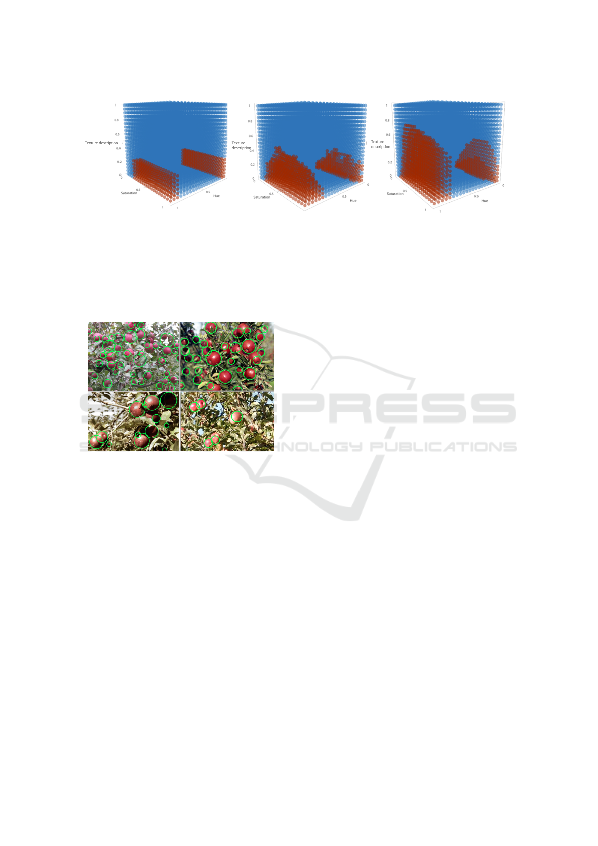
Figure 9: Classiﬁcation of each of the methods for a set of points normalized from 0 to 1 of the 3 characteristics. First is the

decision Tree, then KNN and ﬁnally SVM.

simple decision Tree achieved an overall F-measure

of 62%. Depending on each particular application,

the limitation on the hardware and computational re-

sources, and the requirements on the performance de-

tection, one need to choose the method that better ﬁts

the problem characteristics.

Figure 10: Examples of apples detected. Video and additi-

onal material at (Marzoa, 2017b).

Using the mask of pixels classiﬁed by decision

tree method, morphological operations are applied to

achieve the ﬁnal goal of detecting the apples present

in the test images. Again, part of the images of the

data set were used to train and ﬁt the parameters of

the solution implemented, while other independent

images (never used during the training step) are used

for testing the proposed solution. Figure 10 shows

the output of the proposed solution for four input test

images. As in the pixel classiﬁcation step, the ﬁnal

performance of the proposed solution is analyzed in

therms of the F-measure. It is important to point out

that while the deﬁnition of F-measure, Recall and Pre-

cision is unique, the meaning of this quantities is dif-

ferent in this second step. In the pixel classiﬁcation

step, we deﬁne the TP (true positive) quantity as the

number of pixels classiﬁed as part of an apple that

truly belong to an apple, in the ﬁnal step, TP is deﬁned

as the number of apples correctly detected, while FP

is the number of apples detected that are not present

in the image (false detections) and FN corresponds to

the number of apples present in the image that where

not detected by the method. Table 2 summarizes the

ﬁnal results obtained for the detection of apples. In

this table, the Recall represents the percentage of ap-

ples present in the input image that are correctly de-

tected, and the Precision indicates the percentage of

detections give by the algorithm that actually corre-

spond to an apple. As explained in previous Sections,

Recall and Precision are combined in a single mea-

sure: the F-measure. Others works dont use the same

measurements that us, in general, the focus is on the

over all apple count so we had to calculate the results

that are presented in this table using the images and

results presented in theirs articles.

To conclude this Section is important to highlight

some difﬁculties that arises when comparing different

apple detection approaches. In ﬁrst place, different

solutions proposed in the literature make use of sig-

niﬁcantly different setups. For example: some works

make uses of stereo pairs of cameras plus high preci-

sion positioning systems (Wang et al., 2013), tunnel

like structures (Gongal et al., 2016b) to control illu-

mination conditions, hyperspectral cameras (Safren

et al., 2007), or thermal imaging devices (Stajnko

et al., 2004). Secondly, the conditions of crop yield

also has a great impact on systems performance, for

instance, special fruit thinning may signiﬁcantly sim-

plify the problem. Thirdly, the success measurements

uses also present signiﬁcant variations, for example,

in (Wang et al., 2013) the focus is on the over all

apple count, hence false positive detections may be

compensated with false negative detections (while the

f-measure penalize both).

6 CONCLUSIONS

This article presents a simple pipeline for the de-

tection of apples in crops using pattern recognition

and computer vision tools. The set up consists of a

single RGB camera that captures under unconstrai-

Computer Vision based System for Apple Detection in Crops

247

Table 1: Values of parameters used.

Algorithm Parameter Value

Decision tree Hue min

Hue max

Sat min

Edges density

161

0 - 100

KNN K

% of pixel background

45%

SVM Gamma

100

Morphology Erode

Dilate

Hough circles Min radio

Max radio

Min distance

Accumulator

Post-processing in circles Min area 20%

Table 2: Recall, Precision and F-measure for different apple

detection strategies.

Method Recall Precision F-measure

(Zhao et al., 2005) 67,9% 100,0% 80.1%

(Linker et al., 2012) 72,8% 97,2% 83.3%

(Ji et al., 2012) 46,4% 100,0% 63,4%

ours 92,0% 90,3% 91.5%

ned natural illumination conditions in unthinned ap-

ple crops.

The detection of apples was made in two big sta-

ges. First the classiﬁcation of pixels and then the

detection of apples within the previously classiﬁed

pixels. Three techniques were studied for the clas-

siﬁcation of pixels: decision tree, KNN and SVM.

The best results were obtained with KNN algorithm,

while the decision tree probes to be a very adequate

alternative if computational cost or time are very limi-

ted. The determinant features to make the classiﬁca-

tion were tonality, saturation and edge density. As an

improvement of the recognition of pixels, morpholo-

gical operations were used. Once the pixels had been

classiﬁed, we proceeded to the detection of the apples

by using the Hough transform for circles. Finally, the

quantity of pixels within the circles found was analy-

zed to validate the circles detected and signiﬁcantly

reduce the number of false positive.

The main contributions of this work are: The use

of robust machine learning techniques by facing the

problem as a pattern recognition imbalanced problem.

We present an updated review of the current state of

the art and create a database with 266 high resolution

images which was made publicly available.

There are some evident path in which this work

can be pushed forward. For example: the output of

multiple classiﬁers can be combined to improve the

over all performance (Kuncheva, 2004). With the in-

crease of the number of publicly available databases,

the design of complex modern classiﬁers such as deep

neural networks will be possible. And ﬁnally, instead

of processing individual images, sequence of images

(video data) can be analyzed ensemble exploiting the

temporal correlation of the data.

VISAPP 2018 - International Conference on Computer Vision Theory and Applications

248

REFERENCES

Aggelopoulou, A., Bochtis, D., Fountas, S., Swain, K. C.,

Gemtos, T., and Nanos, G. (2011). Yield prediction in

apple orchards based on image processing. Precision

Agriculture, 12(3):448–456.

Barandela, R., S

anchez, J. S., Garcıa, V., and Rangel, E.

(2003). Strategies for learning in class imbalance pro-

blems. Pattern Recognition, 36(3):849–851.

Bishop, C. M. (2006). Pattern recognition and machine le-

arning. springer.

Brunelli, R. (2009). Template matching techniques in com-

puter vision: theory and practice. John Wiley & Sons.

Di Martino, M., Decia, F., Molinelli, J., and Fern

andez, A.

(2012). Improving electric fraud detection using class

imbalance strategies. In International Conference on

Pattern Recognition and Methods, 1st. ICPRAM., pa-

ges 135–141.

Di Martino, M., Fern

andez, A., Iturralde, P., and Le-

cumberry, F. (2013a). Novel classiﬁer scheme for

imbalanced problems. Pattern Recognition Letters,

34(10):1146–1151.

Di Martino, M., Hern

andez, G., Fiori, M., and Fern

andez,

A. (2013b). A new framework for optimal classiﬁer

design. Pattern Recognition, 46(8):2249–2255.

Dougherty, E. R. and Lotufo, R. A. (2003). Hands-on mor-

phological image processing, volume 59. SPIE press.

Garc

ıa, V., S

anchez, J., and Mollineda, R. (2012). On

the suitability of numerical performance measures for

class imbalance problems. International Conference

In Pattern Recognition Aplications and Methods, pa-

ges 310–313.

Gongal, A., Silwal, A., Amatya, S., Karkee, M., Zhang, Q.,

and Lewis, K. (2016a). Apple crop-load estimation

with over-the-row machine vision system. Computers

and Electronics in Agriculture, 120:26–35.

Gongal, A., Silwal, A., Amatya, S., Karkee, M., Zhang, Q.,

and Lewis, K. (2016b). Apple crop-load estimation

with over-the-row machine vision system. Computers

and Electronics in Agriculture, 120:26–35.

Hearst, M. A., Dumais, S. T., Osuna, E., Platt, J., and Schol-

kopf, B. (1998). Support vector machines. IEEE In-

telligent Systems and their Applications, 13(4):18–28.

Japkowicz, N. and Stephen, S. (2002). The class imbalance

problem: A systematic study. Intelligent data analy-

sis, 6(5):429–449.

Ji, W., Zhao, D., Cheng, F., Xu, B., Zhang, Y., and Wang, J.

(2012). Automatic recognition vision system guided

for apple harvesting robot. Computers & Electrical

Engineering, 38(5):1186–1195.

Jim

enez, A. R., Jain, A. K., Ceres, R., and Pons, J. (1999).

Automatic fruit recognition: a survey and new results

using range/attenuation images. Pattern recognition,

32(10):1719–1736.

Kubat, M., Matwin, S., et al. (1997). Addressing the curse

of imbalanced training sets: one-sided selection. In

ICML, volume 97, pages 179–186. Nashville, USA.

Kuncheva, L. I. (2004). Combining pattern classiﬁers: met-

hods and algorithms. John Wiley & Sons.

Linker, R., Cohen, O., and Naor, A. (2012). Determination

of the number of green apples in rgb images recorded

in orchards. Computers and Electronics in Agricul-

ture, 81:45–57.

Liu, X.-Y., Wu, J., and Zhou, Z.-H. (2009). Exploratory un-

dersampling for class-imbalance learning. IEEE Tran-

sactions on Systems, Man, and Cybernetics, Part B

(Cybernetics), 39(2):539–550.

Manjunath, B. S., Ohm, J.-R., Vasudevan, V. V., and Ya-

mada, A. (2001). Color and texture descriptors. IEEE

Transactions on circuits and systems for video techno-

logy, 11(6):703–715.

Marzoa, C. (2017a). Apple data base. Website. last chec-

ked: 17.07.2017.

Marzoa, C. (2017b). Web of the apple detection proyect.

Website. last checked: 17.07.2017.

Muja, M. and Lowe, D. G. (2009). Fast approximate nearest

neighbors with automatic algorithm conﬁguration. VI-

SAPP (1), 2(331-340):2.

OpenCV (2017). Opencv. Website. last checked:

17.07.2017.

Rakun, J., Stajnko, D., and Zazula, D. (2011). Detecting

fruits in natural scenes by using spatial-frequency ba-

sed texture analysis and multiview geometry. Compu-

ters and Electronics in Agriculture, 76(1):80–88.

Robinson, T. (2006). The evolution towards more competi-

tive apple orchard systems in the usa. In XXVII Inter-

national Horticultural Congress-IHC2006: Internati-

onal Symposium on Enhancing Economic and Envi-

ronmental 772, pages 491–500.

Safren, O., Alchanatis, V., Ostrovsky, V., and Levi, O.

(2007). Detection of green apples in hyperspectral

images of apple-tree foliage using machine vision.

Transactions of the ASABE, 50(6):2303–2313.

Scholkopf, B. and Smola, A. J. (2001). Learning with ker-

nels: support vector machines, regularization, optimi-

zation, and beyond. MIT press.

Stajnko, D., Lakota, M., and Ho

cevar, M. (2004). Estima-

tion of number and diameter of apple fruits in an or-

chard during the growing season by thermal imaging.

Computers and Electronics in Agriculture, 42(1):31–

42.

Szeliski, R. (2010). Computer vision: algorithms and ap-

plications. Springer Science & Business Media.

Tabb, A. L., Peterson, D. L., and Park, J. (2006). Segmen-

tation of apple fruit from video via background mo-

deling. In 2006 ASAE Annual Meeting, page 1. Ameri-

can Society of Agricultural and Biological Engineers.

Wang, Q., Nuske, S., Bergerman, M., and Singh, S. (2013).

Automated crop yield estimation for apple orchards.

In Experimental robotics, pages 745–758. Springer.

Zhao, J., Tow, J., and Katupitiya, J. (2005). On-tree fruit

recognition using texture properties and color data.

In Intelligent Robots and Systems, 2005.(IROS 2005).

2005 IEEE/RSJ International Conference on, pages

263–268. IEEE.

Computer Vision based System for Apple Detection in Crops

249