
Sensor-fusion-based Trajectory Reconstruction for Mobile Devices
Jielei Zhang, Jie Feng and Bingfeng Zhou
Institute of Computer Science and Technology, Peking University, Beijing, China
Keywords:
Inertial Measurement Unit, Sensor Fusion, Inertial Navigation, Trajectory Reconstruction.
Abstract:
In this paper, we present a novel sensor-fusion method that reconstructs trajectory of mobile devices from
MEMS inertial measurement unit (IMU). In trajectory reconstruction, the position estimation suffers seriously
from the errors in the raw MEMS data, e.g. accelerometer signal, especially after its second-order integration
over time. To eliminate the influence of the errors, a new error model is proposed for MEMS devices. The
error model consists of two components, i.e. noise and bias, corresponding to different types of errors. For
the noise component, a low-pass filter with down sampling is applied to reduce the inherent noise in the data.
For the bias component, an algorithm is designed to detect the events of movement in a manner of sensor
fusion. Then, the denoised data is further calibrated, according to different types of events to remove the bias.
We apply our trajectory reconstruction method on a quadrotor drone with low-cost MEMS IMU devices, and
experiments show the effectiveness of the method.
1 INTRODUCTION
The trajectory reconstruction of mobile device is
widely used in applications such as self-localization
and map building (Ten Hagen and Krose, 2002). The
self-location information can provide important cam-
era parameters in 3-D reconstruction (Kopf et al.,
2014) or image-based rendering. Additionally, it can
also be applied in the drone cinematography as virtual
rail (N
¨
ageli et al., 2017). Thus, the trajectory recon-
struction is useful in computer graphics.
An option for trajectory reconstruction is to take
advantage of Inertial Measurement Unit (IMU) car-
ried by mobile devices, from which the position can
be calculated by the second-order integration of ac-
celerometer signals (Suvorova et al., 2012). In this pa-
per, we adopt low-cost MEMS IMU in trajectory re-
construction. Due to insufficient accuracy of MEMS
signals, significant errors may occur in measured data.
The errors are usually caused by the integration of
noise and bias (Woodman, 2007).
A number of methods have been proposed to re-
duce MEMS signal errors (Yang et al., 2004; Pedley,
2013; Fredrikstad, 2016). For instance, Kalman Fil-
ter is a common estimation approach, usually used
in combination with computer vision or GPS data
(Mourikis et al., 2009). But Kalman Filter highly de-
pends on the error-state vector which is calculated in
advance. Hence, large deviation of error-state esti-
mation will lead to poor results. On the other hand,
computer vision or GPS data is not always available.
Vision-based methods have low accuracy in texture-
less or low-illumination environments, while GPS is
not effective in enclosed spaces, such as tunnels.
Because of these limitations, in this paper we fo-
cus on the trajectory reconstruction of mobile devices
on the basis of IMU. An effective method is proposed
to reduce the errors in MEMS sensors.
We adopt an error model consisting of the two
types of MEMS errors: the noise and the bias. Unlike
other methods that treat the error model as a whole,
we process the two components separately to reduce
errors without highly depending on the priori estima-
tion. In the noise component, errors are treated as
high-frequency signals, which can be reduced by a
low-pass filter, combined with down sampling. In the
bias component, errors occur in a form of data drift-
ing. To eliminate this type of errors, we first detect the
events of movement by combining the data of multi-
ple sensors. The accelerometer data is then segmented
into sections by the timestamps of those events, and
the data drifting is corrected in each section.
The pipeline of our method is as follows: First,
IMU sensor data is collected and preprocessed. Then,
we establish the error model to eliminate errors.
The accelerometer data is processed by sections on
the timeline, according to the sensor-fusion algo-
rithm, and result in calibrated accelerometer data. Fi-
nally, the trajectory can be reconstructed through the
second-order integration of the calibrated accelerom-
48
Zhang, J., Feng, J. and Zhou, B.
Sensor-fusion-based Trajectory Reconstruction for Mobile Devices.
DOI: 10.5220/0006532900480058
In Proceedings of the 13th International Joint Conference on Computer Vision, Imaging and Computer Graphics Theory and Applications (VISIGRAPP 2018) - Volume 1: GRAPP, pages
48-58
ISBN: 978-989-758-287-5
Copyright © 2018 by SCITEPRESS – Science and Technology Publications, Lda. All rights reserved

eter data. Experiments results prove the effectiveness
of our method.
The main contributions of this paper include:
1. A novel error model for IMU data is proposed,
so that different types of errors can be eliminated.
This method relies less on priori estimation.
2. Our sensor-fusion-based bias elimination algo-
rithm is highly adaptive. In this paper, we com-
bine accelerometers with gyroscopes and ultra-
sonic sensors. In fact, the type of combined sen-
sors is not limited to those mentioned above. It
can be extended to any other sensors.
3. Our method works effectively even on low-cost
MEMS IMU which often produces more errors,
while most of other methods work on expensive
high-precision IMU.
2 RELATED WORK
2.1 Sensors in Mobile Devices
There are a number of sensors carried by mobile de-
vices which can be used in trajectory reconstruction.
Some commonly used sensors include :
GPS. The principle of GPS-based localization is that,
a GPS receiver monitors several satellites and solves
equations to determine the position of the receiver and
its deviation in real time. Due to the low accuracy of
GPS, Aided Navigation method is raised to improve
accuracy (Farrell, 2008). However, GPS is not avail-
able around large obstacles such as tall buildings and
heavily wooded areas (Kleusberg and Langley, 1990),
and this kind of methods will be invalid in such cases.
Camera. Visual odometry is a process of determining
the position and orientation of a robot by analyzing
the associated camera images (Huang et al., 2017).
There are plenty of methods that adopt camera in tra-
jectory reconstruction. The method in (Pflugfelder
and Bischof, 2010) locates two surveillance cameras
and simultaneously reconstructs object trajectories in
3D space. Silvatti et al. utilizes submerged video
cameras in an underwater 3D motion capture system,
which can reconstruct 3D trajectory (Silvatti et al.,
2013). Nevertheless, cameras are not effective in tex-
tureless environment, such as wide snowfield.
Inertial Measurement Unit (IMU). IMU is an elec-
tronic device, which is a combination of 3-axis ac-
celerometers and 3-axis gyroscopes to measure the
specific force and angular velocity of an object. Ac-
cording to the work of (Titterton and Weston, 2004),
trajectory can be reconstructed through the second-
order integration of the accelerometer signals. Gy-
roscopes are used to obtain the attitude information,
which allows the accelerometer signals to be trans-
formed from the body frame to the inertial frame
(Suh, 2003).
Some work focuses on utilizing the IMU signals
to reconstruct trajectory (Suvorova et al., 2012). For
example, Toyozumi et al. provides a pen tip direction
estimation method and writing trajectory reconstruc-
tion method based on IMU (Toyozumi et al., 2016).
Wang et al. develops an error compensation method
and a multi-axis dynamic switch to minimize the cu-
mulative errors caused by sensors (Wang et al., 2010).
Most mobile devices adopt MEMS IMU, for it
is low-cost and light-weighted. However, the main
weakness of the MEMS IMU is its low accuracy on
account of errors (Park and Gao, 2008).
Wi-Fi / Bluetooth. Localization based on Wi-Fi
/ Bluetooth is mainly applied to indoor situations
(Biswas and Veloso, 2010). A most common localiza-
tion technique with wireless access points measures
the magnitude of the received signals and adopts the
method of “fingerprinting” for getting position infor-
mation (Chen and Kobayashi, 2002). Similar prin-
ciples are also used in Bluetooth-based localization
(Faragher and Harle, 2015). The inconvenience of
this category of approaches is the requirement of set-
ting up base stations in the scene. Hence, the Wi-
Fi/Bluetooth signal is not always available for most
common situations.
Ultrasonic Sensor / LIDAR. The principle of local-
ization through LIDAR (Amzajerdian et al., 2011)
and ultrasonic sensors (Hazas and Hopper, 2006) are
similar. They measure the distance to a certain target
by emitting a pulse and receiving echoes with a sen-
sor. Nonetheless, LIDAR is so expensive that most
mobile devices are not equipped with it, while the
measuring range of ultrasonic sensors is too limited
(Rencken, 1993).
Taking into account the advantages and disadvan-
tages, we employ MEMS IMU as a main source of
data for reconstructing trajectory in our work. MEMS
IMU is commonly equipped in mobile devices, and
hence IMU-based trajectory reconstruction methods
are more practicle. On the other hand, since MEMS
IMU signals often carry large errors, it is impossible
to be used alone for trajectory reconstruct. Therefore,
we design a sensor-fusion algorithm to eliminate er-
rors in IMU signals.
Sensor-fusion-based Trajectory Reconstruction for Mobile Devices
49
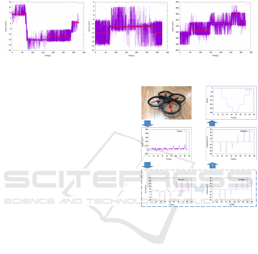
Figure 1: Raw accelerometer signals of 3 axes (X,Y and Z) collected from a static device. The significant noise and data
drifting in the signal will lead to wrong results in trajectory reconstruction.
2.2 IMU Signals
Recent advances in MEMS technique bring possibil-
ity of producing small and light inertial navigation
systems. However, the main disadvantage of MEMS
devices is its low accuracy, which is indicated by bias
and noise in their measurements as elaborated in the
work of Woodman (Woodman, 2007) and illustrated
in Fig.1. During position tracking, the accelerometer
signals are integrated twice, and therefore the errors
grow even rapidly.
Some researchers pay attention to reducing errors
caused by IMU devices. Yang et al. proposes a
zero velocity compensation (ZVC) mechanism to re-
duce the accumulative errors of IMUs (Yang et al.,
2004). Pedley applies linear least squares optimiza-
tion to compute the recalibration parameters from the
available measurements (Pedley, 2013).
Some other methods adopt Kalman Filter com-
bined with computer vision as an assistant of IMU
to improve accuracy. For instance, a VISINAV algo-
rithm is presented to enable planetary landing, utiliz-
ing an extended Kalman filter (EKF) to reduce errors
(Mourikis et al., 2009). In an extended Kalman filter,
a state space model is applied to estimate the naviga-
tion states (Fredrikstad, 2016). However, the error-
state vector, which is estimated in advance, has a di-
rect impact on the result, that is, large deviation of
error-state estimation leads to poor results.
Most of those methods are not designed for low-
cost MEMS devices, which are commonly used in
mobile devices but produce large errors.
Consequently, in this paper, we put emphasis on
the trajectory reconstruction from low-cost MEMS
IMU. A quadrotor drone is taken as an example of
mobile devices. During the course, we design differ-
ent error models for different types of errors, so that
diverse errors can be eliminated in targeted ways.
Error Model
Reducing Noise
Eliminating Bias
1
Preprocess
Mobile Device
Reconstructed trajectory
Calibrated data
2
4
Integration
IMU data
Model Establishment
Error Elimination
Figure 2: The pipeline of our method: 1) Data collection
and preprocessing; 2) Error model establishment; 3) Error
elimination; 4) Integration and trajectory reconstruction.
3 IMU-BASED TRAJECTORY
RECONSTRUCTION
In this paper, we propose a trajectory reconstruction
method for mobile devices, utilizing the measurement
of IMU and other sensors. The pipeline of our method
is illustrated in Fig.2. It consists of four phases:
1. Sensor data collection and preprocess;
2. Error model establishment for the sensor data;
3. Error elimination on the basis of our error model;
4. Trajectory reconstruction through integration of
calibrated accelerometer data.
First, sensor data, mainly including the ac-
celerometer, gyroscope and ultrasonic signals, is col-
lected discretely from the target mobile device. Since
trajectory is reconstructed in the inertial frame while
IMU data is collected in the body frame (Lee et al.,
GRAPP 2018 - International Conference on Computer Graphics Theory and Applications
50

2010), we first perform a coordinate transformation in
a preprocessing phase. We denotes the raw measured
accelerometer data at time point t in the body frame as
a
0
(t) = (a
0
x
(t), a
0
y
(t), a
0
z
(t))
T
, and its correspondence in
the inertial frame as ˜a(t) = ( ˜a
x
(t), ˜a
y
(t), ˜a
z
(t))
T
. Thus,
the coordinate transformation can be formulated as
a
0
(t) = R(φ, θ, ϕ) · ˜a(t), (1)
where R(φ, θ, ϕ) is the rotation matrix from the inertial
frame to the body frame (Bristeau et al., 2011); φ , θ
and ϕ stand for the three Euler angles between the two
frames.
The raw IMU data contains a lot of errors due to
the low accuracy of MEMS. Hence the most impor-
tant step in our pipeline is to eliminate the errors be-
fore the data is used for trajectory calculation.
As mentioned above, errors in MEMS are com-
prised of the noise and the bias. Unlike other methods
which consider the two parts together, we divide the
error model into a noise component
n
(t) and a bias
component
b
(t) in the second step. So we have
˜a(t) = α · a(t) +
n
(t) +
b
(t) − H · g, (2)
where a(t) is the calibrated accelerometer data, α is a
scale factor between the measured inertial data and
the actual data, H = (0, 0, 1)
T
, and g stands for the
gravitational acceleration.
According to this error model. The two parts are
processed separately in the next phase. We first re-
duce the noise, then eliminate the bias, and finally ob-
tain a set of calibrated accelerometer data a(t).
In the last phase, the calibrated accelerometer
data is integrated over time to obtain the 3D trajec-
tory. Hence, the 3D position at time t
i
, noted as
S
i
= (S
ix
, S
iy
, S
iz
)
T
, which is calculated as follows:
S
i
= V
i
∗ ∆t
i
+ S
i−1
=
i
Õ
k=0
v
k
∗ ∆t
k
=
i
Õ
k=0
(
k
Õ
j=0
a(t
j
)∆t
j
)∆t
k
,
(3)
where a(t
i
) represents the ith signal of the calibrated
accelerometer data, and ∆t
i
is the time interval be-
tween t
i
and t
i−1
. V
i
stands for the velocity calculated
from a(t). Thence, {S
i
|i = 1, 2, ..., n} composes the re-
constructed trajectory.
4 REDUCING NOISE
As shown in Fig.1, the measured accelerometer sig-
nals seriously oscillate at a large amplitude around
certain values (marked by red lines). This vibration
results in noise. On the other hand, even when the de-
vice remains still while collecting the signal, the red
1 2
(a) (b)
(c)
Figure 3: Eliminating noise and bias errors in the ac-
celerometer data. (a) Raw measured accelerometer signals
collected from a static devices; (b) After reducing noise; (c)
After eliminaing bias.
line keeps drifting from its true value, and presents a
step shaped line instead of a straight line. This kind
of data drifting is called bias.
The noise in the MEMS IMU data could be re-
garded as a high frequency signal superimposed on
the real signal, which is a low frequency signal.
Therefore, valid data could be obtained by filtering
out the noise through a low-pass filter. Hence, given
the measured raw accelerometer signals { ˜a(t
i
)|i =
1, 2, ..., n}, the denoised accelerometer data { ˆa
0
(t
i
)} is
calculated by
ˆa
0
(t
i
) =
n
Õ
k=0
h(t
k
) ˜a(t
i
− t
k
), (4)
where h(.) is the impulse response function of the
low-pass filter, and the filter is presented in a convo-
lution form in the time domain.
In order to achieve better denoising result, and
to reduce the amount of the following calculation as
well, a down sampling is applied to the filtered data.
Thus, the final denoised accelerometer data set { ˆa(t)}
is a subset of { ˆa
0
(t)}, which is down sampled at a
certain period δ. In our current implementation, we
adopt δ = 100ms.
Since high frequency noise also exists in the sig-
nals of other sensors such as gyroscopes and ultra-
sonic sensors, the data of these sensors can also be
denoised in the similar way. The resulting smoother
data will be used in the following calculation of bias
elimination.
5 ELIMINATING BIAS
After filtering out the noise, we obtain a relatively
smooth curve of the accelerometer data (Fig.3(b)).
However, bias errors still exist. It is reflected as the
data drifting, and is varying over time (Woodman,
2007), as demonstrated by the change of the red lines
in Fig.1. In prior works, the bias is removed only once
before the whole movement, hence we are aiming to
improve this by dynamically eliminate the bias during
the movement.
Through the observation of the data, we found that
it is difficult to determine when the IMU produces
Sensor-fusion-based Trajectory Reconstruction for Mobile Devices
51

Event timestamp
detected
Other sensors
remain static
Static event
Yes
Other sensors
have excep-
tional data
Invalid event
Yes
No
Variation of
other sensors
is small
Bias event
Yes
Movement event
No
No
Figure 4: Determining the type of an event according to the
status of multiple sensors.
a bias by only analyzing the absolute value of ac-
celerometer data. Therefore, a method is needed to
find out the time point when a bias happens, so that
the bias errors can be correctly eliminated during the
movement of the device.
Though bias occurs on all MEMS sensors, it is
less probably to occur on multiple sensors at the same
time. Hence, we may apply a sensor-fusion method
to detect the time point when bias occurs. Accord-
ing to these time points, the denoised accelerometer
data can be segmented into a series of sections along
the timeline. In each section, we consider the device
maintaining the same motion status, and thus the ac-
celerometer value should be a constant. We then take
different strategies to eliminate bias errors according
to different status of each section. The segmentation
on the timeline will effectively compensate for the ac-
cumulation of bias errors over time.
Here, we define each section on the timeline as an
ev ent, and the time index of each segmentation point
as an event timestamp.
5.1 Event Detection
In order to detect the event timestamps, we first in-
spect the derivative of the accelerometer data over
time., which shows the change of the accelerometer
data. If it is greater than a certain threshold τ, that in-
dicates the status of the IMU is being changed, i.e. an
event is happening. Hence, this particular time point
is recorded as an event timestamp, the beginning of a
new event.
However, the initially detected events are not nec-
essarily the bias events that we are aiming to process.
Sometimes, exception events will be detected as well.
To discriminate different types of the events, we refer
to the status of multiple different sensors as an assis-
tant, e.g. gyroscopes and ultrasonic sensors. That is
because the possibility of bias occurring simultane-
ously in multiple sensors is extremely low.
As illustrated in Fig.4, by analyzing the data status
from other sensors, the initial events can be classified
into four types:
(a) Calibrated
(c) Calibrated
a
1
a
4
E1
E2
E3
(b) Calibrated
(a) Calibrated
(c) Movement
a
1
a
2
a
3
E1
E2
E3
(b) Bias
Figure 5: An example of event processing. Accelerometer
data is calibrated by sections according to different event
types.
Bias Event. Bias event is when the device produces
bias errors that need to be corrected. If the variation of
other sensors is small at the event timestamp, i.e., the
accelerometer data has an intense change while other
sensors remain stable, we consider bias occurs to the
accelerometer sensor. Therefore, the event is marked
as a bias event.
Movement Event. This type of event indicates that
the device is in a movement. In this case, the change
of the accelerometer data is caused by a real move-
ment, and other sensors should correspondingly show
reasonable variations.
Static Event. In this case, the mobile device is actu-
ally in a static status, i.e. its accelerometer data and
speed should be zero. That can be deduced by Euler
angles (attitude angles) φ, θ and ϕ of the device. If
the values of the three angles are all near to zero, and
the ultrasonics measurement also has little variation,
the event is regarded as a static event.
Invalid Event. In some special cases, we may en-
counter invalid data, for example, when the value ex-
ceeds the measuring range, or the device is in a vi-
olent shaking. Therefore, if other sensors exhibit an
irregular status, e.g. the gyroscope data vibrates fre-
quently and severely in a very short period, the event
is marked as an invalid event.
Here, bias event and movement event are regarded
as regular types, while static event and invalid event
are considered as exception types, which happens oc-
casionally.
5.2 Processing Algorithm
After detecting the event timestamps, the accelerom-
eter data can be segmented into sections, each corre-
sponding to an event. Then, eliminate bias errors in
each section, according to the type of the event. The
bias elimination algorithm is listed as Algorithm 1.
Here, we denote the calibrated accelerometer
value in the previous section as PreAcc, and the bias
value of current section as BiasV alue, both initialized
as zero.
If the section corresponds to a bias event, that
means although a data drifting is occurring, the mo-
GRAPP 2018 - International Conference on Computer Graphics Theory and Applications
52
Algorithm 1: Bias Elimination Algorithm
Input:
1. Denoised accelerometer data { ˆa(t)|t = 1, 2, ...,n};
2. Detected events {E
i
|i = 1, 2, ..., m};
Output:
1. Calibrated accelerometer data {a(t
i
)|i = 1, 2, ..,n};
Definition:
1. t
i
: the event timestamp of E
i
.
2. median(.): a function returns the median value of
a data set.
3. BiasValue: the bias value of the accelerometer
data, initialized as zero;
4. PreAcc: the calibrated accelerometer data of the
prevoius event, initialized as zero;
Algorithm:
1: for i from 1 to m do
2: if E
i
== static then
3: while t ∈
[
t
i
, t
i+1
)
do
4: a(t) = 0.0
5: PreAcc = 0.0
6: BiasV alue = median( ˆa (t), t ∈
[
t
i
, t
i+1
)
)
7: else if E
i
== invalid then
8: All parameters remain unchanged.
9: else if E
i
== bias then
10: while t ∈
[
t
i
, t
i+1
)
do
11: a(t) = Pr eAcc
12: cur Ac c = median( ˆa(t), t ∈
[
t
i
, t
i+1
)
)
13: BiasV alue = cur Acc − PreAcc
14: else if E
i
== movement then
15: cur Ac c = median( ˆa(t), t ∈
[
t
i
, t
i+1
)
)
16: while t ∈
[
t
i
, t
i+1
)
do
17: a(t) = cur Acc − BiasValue
18: PreAcc = cur Acc − BiasV alue
tion status of the device is not actually changing.
Hence, we correct the accelerometer data in this sec-
tion as the calibrated data in the previous section
(Fig.5 (b)). Meanwhile, the bias value, i.e. the dif-
ference between the measured data and the calibrated
data, is updated and recorded as BiasV alue. It will
be used in the processing of the subsequent sections.
If the section corresponds to a movement event,
the variation of the accelerometer data is caused by
a real movement. Then, the calibrated accelerometer
value can be calculated as the median of the data in
this section subtracting current recorded BiasV alue
(Fig.5 (c)). After that, PreAcc is updated as the same
value for the calculation of the following sections.
In the case of a static event, the device stays still.
Hence, the accelerometer data in this section will be
reset to zero. PreAcc is also cleared to zero, and
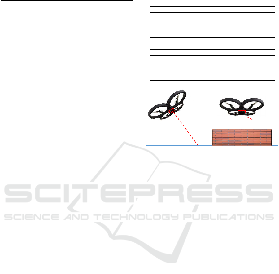
Table 1: Onboard sensors of AR. Drone 2.0.
Sensors Specifications
3-axis accelerometers Bosch BMA 150,
Measuring range: ± 2g
2-axis gyroscopes Invensense IDG500,
Measuring rate: up to 500 deg/s
1-axis gyroscope Epson XV3700,
On vertical axis
Ultrasonic sensor Measuring rate: 25 Hz.
Vertical camera 64
◦
diagonal lens,
Framerate: 60 fps
Front camera 93
◦
wide-angle diagonal lens,
Framerate: 15 fps
ultrasonic
sensors
ultrasonic
sensors
obstacle
(a)
(b)
Figure 6: The ultrasonic measurement may deviate from
the actual height during movement or flying over obstacles.
(The red rectangels stand for the ultrasonic sensor on the
drone, and the red dotted lines indicate the ultrasonic mea-
surements).
the median of the accelerometer data in this section
is recorded as the BiasV alue.
Finally, for an invalid event, it will be ignored.
The process of this event follows the previous event,
and all parameters remain unchanged.
Therefore, the output of the algorithm is the final
calibrated accelerometer data.
6 EXPERIMENTS
So far, we have proposed a trajectory reconstruction
method for mobile devices. The data from the ac-
celerometer and other sensors on the device is utilized
in the reconstruction in a sensor-fusion manner. In
order to validate the effectiveness of our method, we
apply it to a quadrotor drone, which contains low-cost
MEMS IMU and other sensors.
6.1 Implementations
In our experiments, we adopt a Parrot AR. Drone
2.0 as the target mobile device. AR. Drone is a
lightweight quadrotor, equipped with a Linux based
real-time operating system and multiple onboard sen-
sors. The sensors and their specifications are listed
in Table 1. Among all these sensors, accelerometers
Sensor-fusion-based Trajectory Reconstruction for Mobile Devices
53

provide the major data for the calculation of the tra-
jectory, while the others are used as auxiliary sensors
in the bias elimination.
The gyroscope data is used for attitude estimation
and event timestamp detection on the X or Y axis,
because the drone would tilt if there is a movement
on the X - Y plane, and that will result in a variation
of the gyroscope measurement.
On the bottom of the AR. Drone, there is a ul-
trasonic sensor which measures the distance from the
drone to the ground. The derivative of the ultrasonic
data is utilized in event detection on the Z-axis. How-
ever, we do not directly use it as the trajectory on the
Z-axis. That is because when the drone tilts during its
movements, the angle of the ultrasonic sensor would
also change. Therefore, its measurement can not re-
flect the actual height of the drone (Fig.6(a)). Besides,
when the drone flies over obstacles, large variations
may also occur in its measurement (Fig.6(b)).
In addition, we perform our experiments indoor
for the ultrasonic sensor has a limited range. On the
other hand, indoor experiments can also simplify the
flight condition, like the absence of wind.
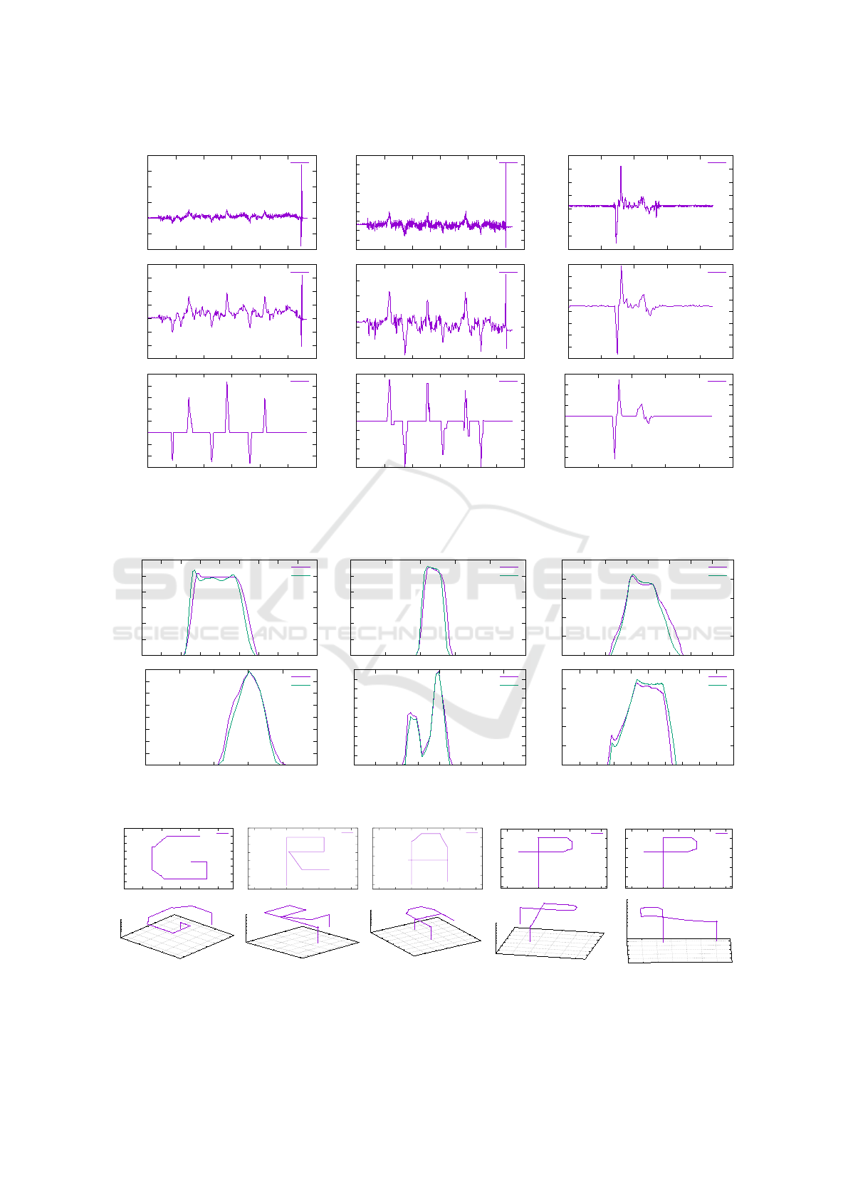
6.2 Experimental Results
In order to verify the effectiveness of the proposed
algorithm, some experiment results are demonstrated
in this section.
Results of Error Elimination. As shown in the first
row of Fig.7, the raw accelerometer data seems to be
out of order because of too much noise and bias. It is
impossible to reconstruct the trajectory through these
raw signals. In the second row, the signals are de-
noised through a low-pass filter and down sampling,
and become smoother, but bias errors still exist. In the
last row is the final calibrated accelerometer data after
bias elimination. Hence, after redundant error signals
are removed and the outliers filter away, valid signals
are extracted by our method.
Trajectory Reconstruction for Single-axis Move-
ments. We first test our trajectory reconstruction
method in relatively simple situations. We make the
drone move in only one direction along X, Y, or Z
axis, and keep invariant in the other two directions.
Therefore, we inspect the data and the motion status
on only one axis, and assume the accelerometer data
on the other two axes are always zero. As shown in
Fig.8, the purple lines are the reconstructed trajecto-
ries by our method, and the green lines are the ground
truth trajectory. We can see that the result is close to
the actual movement. The reconstruction errors are
controlled within 10 cm.
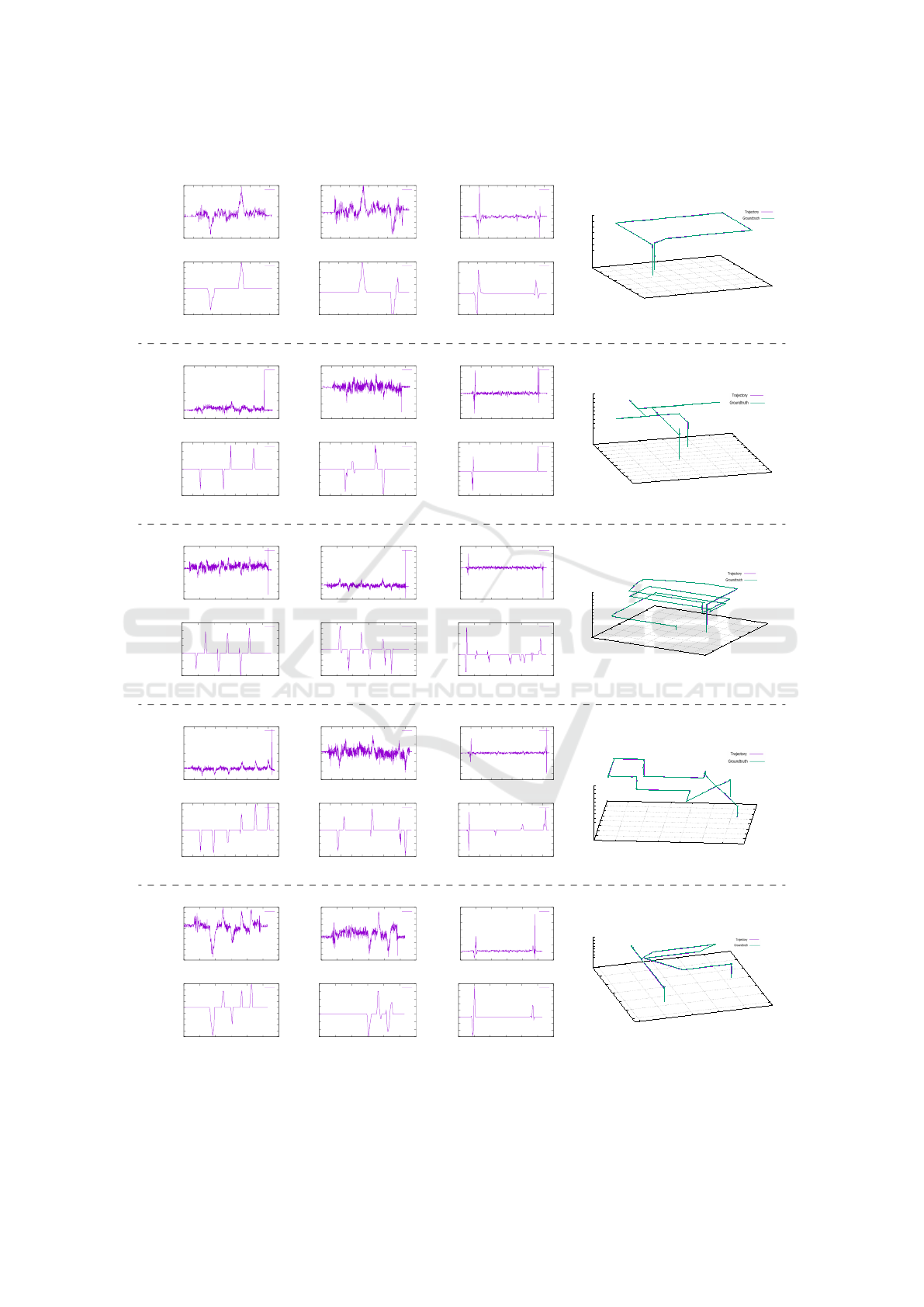
Trajectory Reconstruction for Multiple-axis
Movements. After the single-axis tests, we carry
out more complicated experiments of reconstructing
trajectory on multiple axes. We fly the drone in an
indoor environment, along given routes with various
shapes. The drone is controlled by a flying program,
so that it can fly at a relatively constant speed, and fly
straightly in the given directions.
Several groups of reconstruction results are given
in Fig.9 and Fig.10. We can see that, after denoising
and bias elimination, we can extract valid accelerome-
ter data from the raw signal, and correctly reconstruct
the 3D trajectories of the drone. The reconstructed
trajectories (purple lines) coincide with the ground
truth routes (green lines).
However, due to the instability of the controlling
algorithm inside the drone, the actual flying route of
the drone may have slight offsets. The offsets are too
small to be detected by the low-accuracy onboard sen-
sors, hence they would be ignored by our algorithm.
That is why reconstructed trajectory is a little more
smooth and straight than the actual trajectory.
Adaptive Parameter Adjustment. In order to ob-
tain better results, the event detection thresholds τ for
the accelerometer or other sensors’ data need to be
adjusted to an appropriate value. In fact, this adjust-
ment can be adaptively accomplished in our method.
We first pick a small part of the data at the begin-
ning of the flight, and interactively obtain the optimal
thresholds. Then, the rest of the trajectory can be au-
tomatically reconstructed with these thresholds. An
example is given in Fig.11, the final result is similar
with what we designed in advance. That shows the
adaptability of our method.
7 CONCLUSIONS
In this paper, we present a novel method to recon-
struct trajectory for mobile devices based on low-cost
MEMS IMU, which suffers from low accuracy. To
remove the errors in the raw signals of the IMU and
other sensors, a low-pass filter and down sampling is
applied to reduce the noise, and a sensor-fusion-based
algorithm is used to dynamically eliminate the bias.
Experiments on a quadrotor drone demonstrate that
our method works effectively. This sensor-fusion-
based method can be extended to employ various
kinds of sensors in bias elimination, and hence it is
practical for different mobile devices. Moreover, the
parameter can be adaptively adjusted at the beginning
of the flight.
Currently, one of the limitation of our method is
that it requires relatively flat floor, for complex land-
GRAPP 2018 - International Conference on Computer Graphics Theory and Applications
54
X-axis Y-axis Z-axis
Raw
-400
-200
0
200
400
600
800
0 20 40 60 80 100 120
AccX( cm/s
2
)
Time(s)
Raw accelerometer signal of X-axis
-300
-200
-100
0
100
200
300
400
500
600
700
0 20 40 60 80 100 120
AccY( cm/s
2
)
Time(s)
Raw acceleration signal of Y-axis
-1300
-1200
-1100
-1000
-900
-800
-700
-600
0 5 10 15 20 25
AccZ( cm/s
2
)
Time(s)
Raw accelerometer signal of Z-axis
Denoised
-150
-100
-50
0
50
100
150
200
0 20 40 60 80 100 120
Acc (cm/s
2
)
Time(s)
Accelerometer signal of X-axis after denoising
-150
-100
-50
0
50
100
150
0 20 40 60 80 100 120
Acc (cm/s
2
)
Time(s)
Accelerometer signal of Y-axis after denoising
-1200
-1150
-1100
-1050
-1000
-950
-900
-850
-800
0 5 10 15 20 25
Acc (cm/s
2
)
Time(s)
Acceleration signal of Z-axis after denosing
Calibrated
-60
-40
-20
0
20
40
60
80
100
0 20 40 60 80 100 120
CeliAcc(cm/s
2
)
Time(s)
Accelerometer signal of X-axis after calibration
-100
-80
-60
-40
-20
0
20
40
60
80
100
0 20 40 60 80 100 120
CeliAcc(cm/s
2
)
Time(s)
Accelerometer signal of Y-axis after calibration
-250
-200
-150
-100
-50
0
50
100
150
200
0 5 10 15 20 25
CeliAcc(cm/s
2
)
Time(s)
Accelerometer signal of Z-axis after calibration
Time(s) Time(s) Time(s)
Figure 7: The result of error elimination for the accelerometer data on three axes. The first row is the raw accelerometer data
collected from a quadrotor drone. The second row shows the signal after denoising by a low-pass filter and down sampling.
The last row is the final calibrated output of accelerometer data after bias elimination.
Trajectory(cm)
0
10
20
30
40
50
60
0 2 4 6 8 10 12 14 16 18
Altitude(cm)
Time(s)
Trajectory
ground truth
0
10
20
30
40
50
60
0 5 10 15 20 25
Altitude(cm)
Time(s)
Trajectory
ground truth
0
50
100
150
200
250
0 5 10 15 20 25 30 35 40
Altitude(cm)
Time(s)
Trajectory
ground truth
Trajectory(cm)
0
20
40
60
80
100
120
140
160
0 5 10 15 20 25
Altitude(cm)
Time(s)
Trajectory
ground truth
0
10
20
30
40
50
60
70
80
90
100
0 5 10 15 20 25 30 35 40
Altitude(cm)
Time(s)
Trajectory
ground turth
0
50
100
150
200
250
0 5 10 15 20 25 30 35 40 45 50
Altitude(cm)
Time(s)
Trajectory
ground truth
Time(s) Time(s) Time(s)
Figure 8: Trajectory reconstruction results on a single-axis (purple lines) , comparing with the ground truth(green lines).
-140
-120
-100
-80
-60
-40
-20
0
20
-200 -150 -100 -50 0 50
cm
cm
Traj
0
20
40
60
80
100
120
140
-100 -50 0 50 100 150 200
cm
cm
Traj
0
20
40
60
80
100
120
-100 -50 0 50 100 150 200
cm
cm
Traj
0
50
100
150
200
250
300
-100 -50 0 50 100 150 200
cm
cm
Traj
0
50
100
150
200
250
300
-100 -50 0 50 100 150 200
cm
cm
Traj
-120
-100
-80
-60
-40
-20
0
-50
0
50
100
150
0
10
20
30
40
50
60
70
80
90
100
Z
Traj
X
Y
Z
-120
-100
-80
-60
-40
-20
0
-50
0
50
100
150
0
20
40
60
80
100
120
Z
Traj
X Y
Z
-140
-120
-100
-80
-60
-40
-20
0
20
-100
-50
0
50
100
150
200
-10
0
10
20
30
40
50
60
70
80
90
100
Z
Traj
X
Y
Z
-300
-250
-200
-150
-100
-50
0
50
-100
-50
0
50
100
150
0
20
40
60
80
100
120
140
160
Z
Traj
X
Y
Z
-300
-250
-200
-150
-100
-50
0
50
-100
-50
0
50
100
150
0
20
40
60
80
100
120
140
160
Z
Traj
X
Y
Z
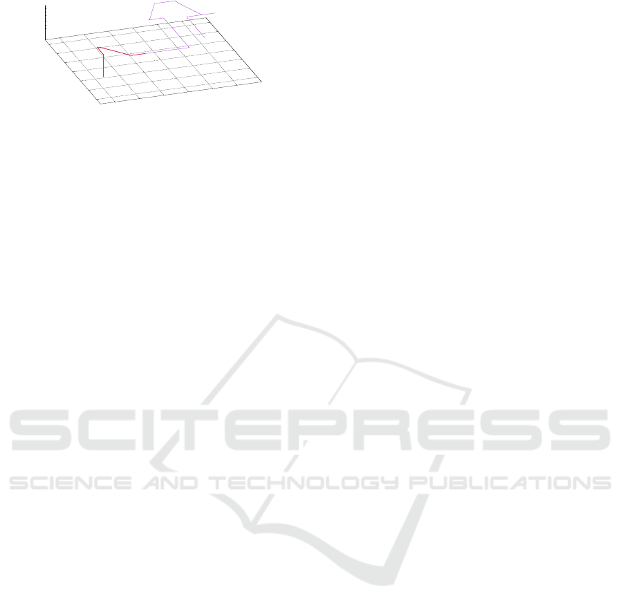
Figure 9: Trajectories reconstructed from Ar.drone. We design target trajectories as the letters of ”GRAPP”. And the results
match the targets well. The first row is the trajectory in X-Y plane. The second row is each corresponding one in three-
dimensional space.
Sensor-fusion-based Trajectory Reconstruction for Mobile Devices
55
X-axis Y-axis Z-axis Reconstructed Trajectory
Raw
-100
-50
0
50
100
150
0 5 10 15 20 25 30 35 40 45 50
AccX( cm/s
2
)
Time(s)
Raw acceleromete r signal of X-axis
-140
-120
-100
-80
-60
-40
-20
0
20
40
60
0 5 10 15 20 25 30 35 40 45 50
AccY( cm/s
2
)
Time(s)
Raw accelerometer signal of Y-axis
-1300
-1200
-1100
-1000
-900
-800
-700
-600
-500
0 5 10 15 20 25 30 35 40 45 50
AccZ( cm/s
2
)
Time(s)
Raw accelerometer signal of Z-axis
-300
-250
-200
-150
-100
-50
0
50
-50
0
50
100
150
200
250
300
350
0
20
40
60
80
100
120
Z (cm)
X (cm)
Y (cm)
Z (cm)
Calibrated
-100
-80
-60
-40
-20
0
20
40
60
80
100
0 5 10 15 20 25 30 35 40 45 50
CeliAcc(cm/s
2
)
Time(s)
Calibrated acceleration data of X-axis
-60
-40
-20
0
20
40
60
80
0 5 10 15 20 25 30 35 40 45 50
CeliAcc(cm/s
2
)
Time(s)
Calibrated acceleration data of Y-axis
-100
-50
0
50
100
150
0 5 10 15 20 25 30 35 40 45 50
CeliAcc(cm/s
2
)
Time(s)
Calibrated acceleration data of Z-axis
Raw
-100
0
100
200
300
400
500
0 10 20 30 40 50 60 70 80 90
AccX( cm/s
2
)
Time(s)
Raw acceleromete r signal of X-axis
-250
-200
-150
-100
-50
0
50
100
0 10 20 30 40 50 60 70 80 90
AccY( cm/s
2
)
Time(s)
Raw acceleromete r signal of Y-axis
-1400
-1300
-1200
-1100
-1000
-900
-800
-700
-600
-500
0 10 20 30 40 50 60 70 80 90
AccZ( cm/s
2
)
Time(s)
Raw acceleromete r signal of Z-axis
-70
-60
-50
-40
-30
-20
-10
0
10
20
30
40
-150
-100
-50
0
50
100
150
0
10
20
30
40
50
60
70
80
Z (cm)
Trajectory
groundtruth
X (cm)
Y (cm)
Z (cm)
Calibrated
-60
-40
-20
0
20
40
60
0 10 20 30 40 50 60 70 80 90
CeliAcc(cm/s
2
)
Time(s)
Calibrated acceleration data of X-axis
-80
-60
-40
-20
0
20
40
60
80
0 10 20 30 40 50 60 70 80 90
CeliAcc(cm/s
2
)
Time(s)
Calibrated acceleration data of Y-axis
-250
-200
-150
-100
-50
0
50
100
150
200
250
300
0 10 20 30 40 50 60 70 80 90
CeliAcc(cm/s
2
)
Time(s)
Calibrated acceleration data of Z-axis
Raw
-200
-150
-100
-50
0
50
100
150
0 20 40 60 80 100 120
AccX( cm/s
2
)
Time(s)
Raw acceleromete r signal of X-axis
-300
-200
-100
0
100
200
300
400
500
600
700
0 20 40 60 80 100 120
AccY( cm/s
2
)
Time(s)
Raw acceleromete r signal of Y-axis
-1800
-1600
-1400
-1200
-1000
-800
-600
-400
0 20 40 60 80 100 120
AccZ( cm/s
2
)
Time(s)
Raw acceleromete r signal of Z-axis
-120
-100
-80
-60
-40
-20
0
20
40
60
-100
0
100
200
300
400
500
600
0
50
100
150
200
250
300
350
400
450
Z (cm)
Trajectory
groundtruth
X (cm)
Y (cm)
Z (cm)
Calibrated
-60
-40
-20
0
20
40
60
80
0 20 40 60 80 100 120
CeliAcc(cm/s
2
)
Time(s)
Calibrated acceleration data of X-axis
-100
-80
-60
-40
-20
0
20
40
60
80
100
0 20 40 60 80 100 120
CeliAcc(cm/s
2
)
Time(s)
Calibrated acceleration data of Y-axis
-100
-50
0
50
100
150
0 20 40 60 80 100 120
CeliAcc(cm/s
2
)
Time(s)
Calibrated acceleration data of Z-axis
Raw
-100
0
100
200
300
400
500
0 10 20 30 40 50 60 70 80 90
AccX( cm/s
2
)
Time(s)
Raw acceleromete r signal of X-axis
-200
-150
-100
-50
0
50
100
0 10 20 30 40 50 60 70 80 90
AccY( cm/s
2
)
Time(s)
Raw acceleromete r signal of Y-axis
-1800
-1600
-1400
-1200
-1000
-800
-600
-400
-200
0 10 20 30 40 50 60 70 80 90
AccZ( cm/s
2
)
Time(s)
Raw acceleromete r signal of Z-axis
-300
-250
-200
-150
-100
-50
0
50
-100
-80
-60
-40
-20
0
20
40
60
-20
0
20
40
60
80
100
120
140
160
Z (cm)
Trajectory
groundtruth
X (cm)
Y (cm)
Z (cm)
Calibrated
-80
-60
-40
-20
0
20
40
60
80
0 10 20 30 40 50 60 70 80 90
CeliAcc(cm/s
2
)
Time(s)
Calibrated acceleration data of X-axis
-80
-60
-40
-20
0
20
40
60
80
0 10 20 30 40 50 60 70 80 90
CeliAcc(cm/s
2
)
Time(s)
Calibrated acceleration data of Y-axis
-200
-150
-100
-50
0
50
100
150
200
0 10 20 30 40 50 60 70 80 90
CeliAcc(cm/s
2
)
Time(s)
Calibrated accel eration data of Z-axis
Raw
-120
-100
-80
-60
-40
-20
0
20
40
60
80
0 10 20 30 40 50 60
AccX( cm/s
2
)
Time(s)
Raw acceleromete r signal of X-axis
-140
-120
-100
-80
-60
-40
-20
0
20
40
0 10 20 30 40 50 60
AccY( cm/s
2
)
Time(s)
Raw acceleromete r signal of Y-axis
-1200
-1000
-800
-600
-400
-200
0
200
0 10 20 30 40 50 60
AccZ( cm/s
2
)
Time(s)
Raw acceleromete r signal of Z-axis
-300
-250
-200
-150
-100
-50
0
-50
0
50
100
150
200
-20
0
20
40
60
80
100
120
Z (cm)
Trajectory
groundtruth
X (cm)
Y (cm)
Z (cm)
Calibrated
-100
-80
-60
-40
-20
0
20
40
60
80
0 10 20 30 40 50 60
CeliAcc(cm/s
2
)
Time(s)
Calibrated acceleration data of X-axis
-60
-40
-20
0
20
40
60
80
0 10 20 30 40 50 60
CeliAcc(cm/s
2
)
Time(s)
Calibrated acceleration data of Y-axis
-150
-100
-50
0
50
100
150
200
250
0 10 20 30 40 50 60
CeliAcc(cm/s
2
)
Time(s)
Calibrated acceleration data of Z-axis
Figure 10: Multi-axis trajectory reconstruction results. In each group, the left three columns show the raw and calibrated
accelerometer data on X, Y and Z axis. The last column illustrates the final 3D reconstructed trajectories of the drone (purple
line), comparing with the ground truth (green line).
GRAPP 2018 - International Conference on Computer Graphics Theory and Applications
56
-100
-80
-60
-40
-20
0
20
0
50
100
150
200
250
300
70
60
50
40
30
20
10
0
X
Y
Z
Figure 11: Adaptive parameter adjustment. Optimal param-
eters are interactively searched for using the first part of data
(red line), and then the whole trajectory (purple line) can be
automatically reconstructed.
scape will influence the output of ultrasonic senor. In
the future work, combining with more sensors, tra-
jectory can be reconstructed in more complicated en-
vironment. Besides, our method does better in re-
constructing straight lines than in curves. However,
curves can be divided into short line segments, hence
theoretically our approach is feasible in reconstruct-
ing trajectory in arbitrary shapes. Note that the flight
route of the drone are not as perfect as our design,
because it will be influenced by the environment and
battery power.
Our trajectory reconstruction method can be ap-
plied in various applications. Since the trajectory can
provide important view point information, 3D recon-
struction, map building or stereoscopic video synthe-
sizing may be potential future research directions.
ACKNOWLEDGEMENTS
This work is partially supported by NSFC grants
#61370112 and #61602012, and the Key Labora-
tory of Machine Perception (Ministry of Education),
Peking University.
REFERENCES
Amzajerdian, F., Pierrottet, D., Petway, L., Hines, G., and
Roback, V. (2011). Lidar systems for precision navi-
gation and safe landing on planetary bodies. In Proc.
SPIE, volume 8192, page 819202.
Biswas, J. and Veloso, M. (2010). Wifi localization and
navigation for autonomous indoor mobile robots. In
Robotics and Automation (ICRA), 2010 IEEE Inter-
national Conference on, pages 4379–4384.
Bristeau, P.-J., Callou, F., Vissiere, D., and Petit, N.
(2011). The navigation and control technology inside
the ar. drone micro uav. IFAC Proceedings Volumes,
44(1):1477–1484.
Chen, Y. and Kobayashi, H. (2002). Signal strength based
indoor geolocation. In Communications, 2002. ICC
2002. IEEE International Conference on, volume 1,
pages 436–439.
Faragher, R. and Harle, R. (2015). Location fingerprint-
ing with bluetooth low energy beacons. IEEE journal
on Selected Areas in Communications, 33(11):2418–
2428.
Farrell, J. (2008). Aided navigation: GPS with high rate
sensors.
Fredrikstad, T. E. N. (2016). Vision aided inertial naviga-
tion. Master’s thesis, NTNU.
Hazas, M. and Hopper, A. (2006). Broadband ultrasonic lo-
cation systems for improved indoor positioning. IEEE
Transactions on mobile Computing, 5(5):536–547.
Huang, A. S., Bachrach, A., Henry, P., Krainin, M., Matu-
rana, D., Fox, D., and Roy, N. (2017). Visual odome-
try and mapping for autonomous flight using an rgb-d
camera. In Robotics Research, pages 235–252.
Kleusberg, A. and Langley, R. B. (1990). The limitations of
gps. GPS World, 1(2).
Kopf, J., Cohen, M. F., and Szeliski, R. (2014). First-person
hyper-lapse videos. ACM Transactions on Graphics
(TOG), 33(4):78.
Lee, T., Leoky, M., and McClamroch, N. H. (2010). Ge-
ometric tracking control of a quadrotor uav on se (3).
In Decision and Control (CDC), 2010 49th IEEE Con-
ference on, pages 5420–5425.
Mourikis, A. I., Trawny, N., Roumeliotis, S. I., Johnson,
A. E., Ansar, A., and Matthies, L. (2009). Vision-
aided inertial navigation for spacecraft entry, de-
scent, and landing. IEEE Transactions on Robotics,
25(2):264–280.
N
¨
ageli, T., Meier, L., Domahidi, A., Alonso-Mora, J., and
Hilliges, O. (2017). Real-time planning for automated
multi-view drone cinematography. ACM Transactions
on Graphics (TOG), 36(4):132.
Park, M. and Gao, Y. (2008). Error and performance analy-
sis of mems-based inertial sensors with a low-cost gps
receiver. Sensors, 8(4):2240–2261.
Pedley, M. (2013). High precision calibration of a three-axis
accelerometer. Freescale Semiconductor Application
Note, 1.
Pflugfelder, R. and Bischof, H. (2010). Localization and
trajectory reconstruction in surveillance cameras with
nonoverlapping views. IEEE Transactions on Pattern
Analysis and Machine Intelligence, 32(4):709–721.
Rencken, W. D. (1993). Concurrent localisation and map
building for mobile robots using ultrasonic sensors. In
IROS’93. Proceedings of the 1993 IEEE/RSJ Interna-
tional Conference on, volume 3, pages 2192–2197.
Silvatti, A. P., Cerveri, P., Telles, T., Dias, F. A., Baroni, G.,
and Barros, R. M. (2013). Quantitative underwater
3d motion analysis using submerged video cameras:
accuracy analysis and trajectory reconstruction. Com-
puter methods in biomechanics and biomedical engi-
neering, 16(11):1240–1248.
Suh, Y. S. (2003). Attitude estimation using low cost ac-
celerometer and gyroscope. In Science and Technol-
ogy, 2003. Proceedings KORUS 2003. The 7th Korea-
Russia International Symposium on, volume 2, pages
423–427.
Suvorova, S., Vaithianathan, T., and Caelli, T. (2012).
Action trajectory reconstruction from inertial sensor
Sensor-fusion-based Trajectory Reconstruction for Mobile Devices
57

measurements. In Information Science, Signal Pro-
cessing and their Applications (ISSPA), 2012 11th In-
ternational Conference on, pages 989–994.
Ten Hagen, S. and Krose, B. (2002). Trajectory re-
construction for self-localization and map building.
In Robotics and Automation, 2002. Proceedings.
ICRA’02. IEEE International Conference on, vol-
ume 2, pages 1796–1801.
Titterton, D. and Weston, J. L. (2004). Strapdown inertial
navigation technology, volume 17.
Toyozumi, N., Takahashi, J., and Lopez, G. (2016). Trajec-
tory reconstruction algorithm based on sensor fusion
between imu and strain gauge for stand-alone digi-
tal pen. In Robotics and Biomimetics (ROBIO), 2016
IEEE International Conference on, pages 1906–1911.
Wang, J.-S., Hsu, Y.-L., and Liu, J.-N. (2010). An inertial-
measurement-unit-based pen with a trajectory recon-
struction algorithm and its applications. IEEE Trans-
actions on Industrial Electronics, 57(10):3508–3521.
Woodman, O. J. (2007). An introduction to inertial nav-
igation. Technical report, University of Cambridge,
Computer Laboratory.
Yang, J., Chang, W., Bang, W.-C., Choi, E.-S., Kang, K.-
H., Cho, S.-J., and Kim, D.-Y. (2004). Analysis and
compensation of errors in the input device based on
inertial sensors. In Information Technology: Coding
and Computing, 2004. Proceedings. ITCC 2004. In-
ternational Conference on, volume 2, pages 790–796.
GRAPP 2018 - International Conference on Computer Graphics Theory and Applications
58
