Dynamic Pricing Strategies in a Finite Horizon Duopoly

with Partial Information

Rainer Schlosser and Keven Richly

Hasso Plattner Institute, University of Potsdam, Potsdam, Germany

Keywords:

Dynamic Pricing, Duopoly Competition, Response Strategies, Hidden Markov Model, Heuristics.

Abstract:

In many applications the sale of perishable products is characterized by competitive settings and incomplete

information. While prices of sellers are typically observable, the inventory levels of ﬁrms are mutually not

observable. In this paper, we analyze stochastic dynamic pricing models in a ﬁnite horizon duopoly with

partial information. We use a Hidden Markov Model approach to compute strategies that are applicable when

the competitor’s inventory level is not observable. Our approach utilizes feedback pricing strategies that

are optimal if the competitor’s inventory level is observable. We show that price reactions are balancing

two effects: (i) to slightly undercut the competitor’s price to sell more items, and (ii) to use high prices to

promote a competitor’s run-out and to act as a monopolist for the rest of the time horizon. Moreover, we

compute heuristic strategies that can be applied when the number of competitors is large and their strategies

are unknown. We ﬁnd that expected proﬁts are hardly affected by different information structures as long as

the ﬁrms’ information is symmetric.

1 INTRODUCTION

In many markets, ﬁrms offering their products have to

deal with competition and limited information. Sell-

ers are required to choose appropriate pricing de-

cisions to maximize their expected proﬁts. In e-

commerce, it has become easy to observe and to

change prices. Hence, dynamic pricing strategies that

take into account the competitor’s strategies will be

more and more applied.

However, optimal price reactions are not easy to

ﬁnd. Applications can be found in a variety of con-

texts that involve perishable (e.g., airline tickets, ac-

commodation services, seasonal products) as well as

durable goods (e.g., technical devices, natural re-

sources).

In this paper, we study duopoly pricing models in

a stochastic dynamic framework. We focus on per-

ishable goods. In our model, sales probabilities are

allowed to be an arbitrary function of time and the

competitor’s prices. Our aim is to take into account

scenarios in which (i) the competitor’s inventory level

is observable, (ii) the competitor’s inventory level is

not observable, and (iii) even the competitor’s pricing

strategy is unknown.

The best way to sell products is a classical appli-

cation of revenue management theory. The problem is

closely related to the ﬁeld of dynamic pricing, which

is summarized in the books by Talluri, van Ryzin

(2004), Phillips (2005), and Yeoman, McMahon-

Beattie (2011). The survey by Chen, Chen (2015)

provides an excellent overview of recent pricing mod-

els under competition.

In the article by Gallego, Wang (2014) the authors

consider a continuous time multi-product oligopoly

for differentiated perishable goods. They use opti-

mality conditions to reduce the multi-dimensional dy-

namic pure pricing problem to a one dimensional one.

Gallego, Hu (2014) analyze structural properties of

equilibrium strategies in more general oligopoly mod-

els for the sale of perishable products. Martinez-

de-Albeniz, Talluri (2011) consider duopoly and

oligopoly pricing models for identical products. They

use a general stochastic counting process to model the

demand of customers.

Further related models are studied by Yang, Xia

(2013) and Wu, Wu (2015). Dynamic pricing mod-

els under competition that also include strategic cus-

tomers are analyzed by Levin et al. (2009) and Liu,

Zhang (2013). Competitive pricing models with lim-

ited demand information are studied by Tsai, Hung

(2009), Adida, Perakis (2010), and Chung et al.

(2012) using robust optimization and demand learn-

ing approaches. The effects of strategic interaction of

Schlosser, R. and Richly, K.

Dynamic Pricing Strategies in a Finite Horizon Duopoly with Partial Information.

DOI: 10.5220/0006529900210030

In Proceedings of the 7th International Conference on Operations Research and Enterprise Systems (ICORES 2018), pages 21-30

ISBN: 978-989-758-285-1

data-driven strategies in competitive settings are stud-

ied by, e.g., Serth et al. (2017), using an interactive

simulation platform.

In most existing models strong assumptions are

made: (i) sales probabilities are assumed to be of a

highly stylized form, (ii) the competitors’ inventory

levels are assumed to be observable, and (iii) com-

petitors adjust their prices at the same point in time.

While many papers concentrate on (the existence of)

equilibrium strategies, we look for applicable solution

algorithms that allow to compute effective response

strategies in more realistic settings: Demand proba-

bilities are allowed to generally depend on time as

well as the prices of all market participants. Inven-

tory levels do not have to be mutually observable. As

in many practical applications, we assume sequential

mutual price reactions with some delay. We consider

a discrete time model which is based on the inﬁnite

horizon model by Schlosser, Boissier (2017). We ex-

tend their model by limited inventory levels as well as

a ﬁnite horizon setting.

The main contribution of this paper is threefold.

We (i) derive optimal pricing strategies when the com-

petitor’s inventory level is observable, (ii) derive near-

optimal pricing strategies for the case that the com-

petitor’s inventory level is not observable, and (iii)

we present a heuristic for the case that competitors’

strategies are not known.

This paper is organized as follows. In Section 2,

we describe the stochastic dynamic duopoly model

for the sale of a ﬁnite number of perishable goods. We

allow sales intensities to depend on the competitor’s

price as well as on time (seasonal effects). The state

space of our model is characterized by time and the

current competitors’ prices. The stochastic dynamic

control problem is expressed in discrete time.

In Section 3, we consider a duopoly competition,

in which the inventory level of the competitor is ob-

servable. We assume that both competitors act ratio-

nally. We set up a ﬁrm’s Hamilton-Jacobi-Bellman

equation and use recursive methods (value iteration)

to compute both ﬁrms’ value functions. Finally, we

are able to compute optimal feedback prices as well as

expected proﬁts of the two competing ﬁrms. By using

numerical examples, we investigate typical properties

of optimal pricing policies.

In Section 4, we analyze response strategies for

cases where the inventory level of the competitor is

not observable. Using a Hidden Markov Model, we

show how to compute efﬁcient pricing strategies and

how to evaluate expected proﬁts. Our proposed solu-

tion approach is based on the results of the full infor-

mation model introduced in the previous section. The

key idea is to let the competing ﬁrms mutually esti-

mate their competitor’s remaining inventory level. In

Section 5, we show how to derive applicable dynamic

pricing heuristics for cases in which the competitor’s

inventory level as well as its pricing strategy are com-

pletely unknown.

Finally, in Section 6, we compare the different

strategies derived in this paper. Conclusions are of-

fered in the ﬁnal section.

2 MODEL DESCRIPTION

We consider the situation in which a ﬁrm wants to sell

a ﬁnite number of goods (e.g., airline tickets, hotel

tickets, etc.) on a digital market platform. We assume

that a second seller competes for the same market. In

our model, we allow customers to compare prices of

the two different competitors.

The initial number of items of ﬁrm 1 and ﬁrm 2 are

denoted by N

(1)

and N

(2)

, respectively, N

(1)

(2)

∞. We assume that items cannot be reproduced or

reordered. The time horizon T is ﬁnite, T < ∞. If

ﬁrm k sells one item shipping costs c

(k)

have to be

paid, k = 1, 2. A sale of one of ﬁrm k’s items at price

a leads to a net revenue of a −c

(k)

. Discounting is also

included in the model. For the length of one period we

use the discount factor δ, 0 < δ ≤ 1..

Due to customer choice the sales probabilities of

a ﬁrm should depend on its offer price a and the com-

petitor’s price p. We also allow the sales probabilities

to depend on time.

The (joint) probability that between time t and

t +∆ ﬁrm 1 can sell exactly i items at a price a, a ≥ 0,

while ﬁrm 2 can sell j items at price p, p ≥ 0, is de-

noted by, 0 ≤ t < T , i, j = 0,1,2,..., ∆ > 0,

(∆)

(i, j, a, p)

Without loss of generality, in the following, we

assume Poisson distributed sales probabilities, i.e.,

(∆)

(i, j, a, p) :=

(1)

t,∆

(a, p)

· e

−Λ

(1)

t,∆

(a,p)

(2)

t,∆

(p,a)

· e

−Λ

(2)

t,∆

(p,a)

, (1)

where Λ

(k)

t,∆

(a, p) :=

t+∆

(k)

(a, p)ds, k = 1,2, a, p ≥

0; the sales intensity of a ﬁrm k’s product is denoted

by λ

(k)

. In our model, the sales intensity of ﬁrm k,

k = 1, 2, t = [0,T ], a ≥ 0, p ≥ 0,

(k)

(a, p) (2)

is a general function of time t, offer price a, and the

competitor’s price p. The random inventory level

ICORES 2018 - 7th International Conference on Operations Research and Enterprise Systems

of ﬁrm k at time t is denoted by X

(k)

, 0 ≤ t ≤

T . The end of sale for ﬁrm k is the random time

(k)

, when all of its items are sold, that is τ

(k)

min

0≤t≤T

t : X

(k)

= 0

∧ T ; for all remaining t ≥ τ

we let a ﬁrm’s price a

:= 0 and λ

(k)

(0,·) := 0, k =

1,2. As long as a ﬁrm has items left to sell, for each

period t, a price a has to be chosen.

We call strategies (a

)

admissible if they belong

to the class of Markovian feedback policies; i.e., pric-

ing decisions a

≥ 0 may depend on time t, the current

own inventory level, the current prices of the competi-

tor, and (if observable) the inventory level of the com-

petitor. By A we denote the set of admissible prices.

A list of variables and parameters is given in the Ap-

pendix, see Table 5.

In some applications, sellers are able to anticipate

transitions of the market situation. In particular, the

price responses of competitors as well as their reac-

tion time can be taken into account. In this case,

a change of the competitor’s price p can take place

within one period. A typical scenario is that a com-

petitor adjusts its price in response to our price adjust-

ment with a certain delay.

In the following two sections, we assume that the

pricing strategy and the reaction time of competitors

are known; i.e., we assume that choosing a price a at

time t is followed by a state transition (e.g., a competi-

tor’s price reaction) and the current price p changes to

a subsequent price reaction, which may depend on the

current price decision a.

We assume that the state of the system is charac-

terized by the inventory levels of both ﬁrms and the

current competitor’s price. In real-life applications, a

ﬁrm is not able to adjust its prices immediately after

the price reaction of the competing ﬁrm. Hence, we

assume that in each period the price reaction of the

competing ﬁrm takes place with a delay of h periods,

0 < h < 1. I.e., after an interval of size h the competi-

tor adjusts its price, see Figure 1.

Thus in period t the probability to sell exactly i

items during the ﬁrst interval of size h, i.e., [t,t + h],

is P

(h)

(i, j, a

, p

t−1+h

), t = 0,1,...,T − 1. Due to

the competitor’s price reaction for the rest of the

period [t + h,t + 1] the sales probability changes to

(1−h)

t+h

(i, j, a

, p

t+h

), t = 0,1,...,T − 1.

For single intervals [0,h] and [T,T + h], we

assume that there is no demand and we let

(h)

(i, j, a

, p

) = P

(h)

(i, j, a

, p

T −1+h

) := 1

{i= j=0}

The evolution of the cumulated proﬁts of ﬁrm k,

k = 1, 2, is connected to its inventory process X

(k)

and

characterized by each period’s realized net revenues.

Depending on the chosen pricing strategy (a

)

of ﬁrm

1 and the strategy (p

)

of ﬁrm 2, the random accu-

t h

T h

− +

t h

− +

−

T h

− +

Figure 1: Sequence of price reactions in a duopoly with

response time h, 0 < h < 1.

mulated proﬁt of ﬁrm k from time t on (discounted on

time t) amounts to, 0 ≤ t ≤ T , k = 1,2,

(k)

T −1

∑

s=t

s−t

· (a

− c

(k)

) ·



(k)

− X

(k)

s+1



. (3)

Each ﬁrm k seeks to determine a non-anticipating

(Markovian) pricing policy that maximizes its ex-

pected total proﬁt, k = 1, 2,



(k)



(1)

= N

(1)

(2)

= N

(2)



. (4)

In the following sections, we will solve dynamic

pricing problems that are related to (1) - (4). In the

next section, we consider competitive duopoly mar-

kets with complete information. In Section 4, we

compute pricing strategies for scenarios with incom-

plete information and partially observable states, i.e.,

we assume that the competitor’s inventory level is not

observable. In Section 5, we additionally assume that

the competitor’s strategy is unknown. In Section 6,

we compare the results of the three different models.

3 OPTIMAL DYNAMIC PRICING

STRATEGIES IN A DUOPOLY

WITH OBSERVABLE STATES

3.1 Solution with Full Knowledge

In this section, we want to derive mutual optimal price

response strategies. We assume that both ﬁrms can

mutually observe their inventory levels. Following

the Bellman approach, the best expected future prof-

its of ﬁrm 1 and ﬁrm 2, i.e., E(G

(1)

= n,X

(2)

m,p

= p) and E(G

(2)

t+h

(1)

t+h

= n,X

(2)

t+h

= m,a

t+h

= a),

respectively, cf. (4), are described by the value func-

tions V

∗

(n,m, p) and W

∗

t+h

(n,m,a), t = 0, 1, ..., T . The

set of admissible prices A can be continuous or dis-

crete. If either all items are sold or the time is up,

no future proﬁts can be made, i.e., the natural bound-

ary condition for the value functions V and W are

given by, n = 0,1,...,N

(1)

, m = 0, 1, ..., N

(2)

, a, p ∈ A,

t = 0,1,...,T − 1,

∗

(0,m, p) = 0, and V

∗

(n,m, p) = 0, (5)

Dynamic Pricing Strategies in a Finite Horizon Duopoly with Partial Information

∗

t+h

(n,0,a) = 0, and W

∗

T +h

(n,m,a) = 0. (6)

We assume that in case of a run-out a ﬁrm sets

its price equal to zero for the rest of the time horizon.

The Hamilton-Jacobi-Bellman (HJB) equation of ﬁrm

1 can be written as, t = 0, 1, ...,T − 1, n = 1, ..., N

(1)

m = 0,...,N

(2)

, 0 < h < 1, a, p ∈ A,

∗

(n,m, p) = max

a∈A

(

∑

, j

≥0

(h)

, j

,a, p)

∑

, j

≥0

(1−h)

t+h



, j

{n−i

>0}

· a,

∗

t+h



(n − i

)

,(m − j

)

{n−i

>0}

· a





(a − c

(1)

) · min(n,i

+ i

+δ·V

∗

t+1



(n − i

− i

)

,(m − j

− j

)

{m− j

− j

>0}

·p

∗

t+h



(n − i

)

,(m − j

)

{n−i

>0}

· a



. (7)

Note, (7) mirrors all possible sales scenarios

within one period of time and takes the corresponding

inventory transitions as well as the anticipated optimal

price reactions of the competitor into account.

The HJB of ﬁrm 2 is given by, t = 0,1, ..., T − 1,

n = 0,...,N

(1)

, m = 1,...,N

(2)

, 0 < h < 1, a, p ∈ A,

∗

t+h

(n,m,a) = max

p∈A

(

∑

, j

≥0

(1−h)

t+h

, j

,a, p)

∑

, j

≥0

(h)

t+1

, j

∗

t+1



(n − i

)

,(m − j

)

{m− j

>0}

· p



{m− j

>0}

· p





(p − c

(2)

) · min(m, j

+ j

+δ ·W

∗

t+1+h



(n − i

− i

)

,(m − j

− j

)

{n−i

−i

>0}

·a

∗

t+1



(n − i

)

,(m − j

)

{m− j

>0}

· p



. (8)

The associated prices of both ﬁrms are given by

the arg max of (7) and (8), respectively, i.e., n, m > 0,

t = 0,1,...,T − 1,

∗

(n,m, p) = argmax

a∈A

{

...

}

, (9)

∗

t+h

(n,m,a) = argmax

p∈A

{

...

}

. (10)

If a ﬁrm runs out of inventory, we set the price 0,

i.e., for all m, p we let a

∗

(0,m, p) = 0 and for all n, a,

we let p

∗

t+h

(n,0,a) = 0. The coupled value functions

and the optimal feedback policies of the two compet-

ing ﬁrms can be computed in the following recursive

order:

∗

T −1+h

(n,m,a),W

∗

T −1+h

(n,m,a) →

∗

T −1

(n,m, p),V

∗

T −1

(n,m, p)→ . . .

...→ p

∗

(n,m,a),W

∗

(n,m,a)

→a

∗

(n,m, p),V

∗

(n,m, p). (11)

3.2 Numerical Examples

To illustrate the approach, cf. (7) - (11), in the

following, we consider a numerical example.

Example 3.1. We assume a duopoly. Let T = 50,

(1)

= c

(2)

= 10, N

(1)

= N

(2)

= 10, δ = 1, h = 0.5,

and a ∈ A := (10,20,...,400). We assume Poisson

distributed sales probabilities P

(h)

(i, j, a, p), which

are determined by t = 0, h, 1, ..., T , k = 1,2, cf. (1),

(k)

t,h

(a, p) := h ·



1 − e

−10

·a

−2.5+t/T



· β(a, p), and the

factor β(a, p) :=

{a>0}

·(p−L·min(a,p))

a+p−2·L·min(a,p)

, L := 0.8 < 1.

Table 1 illustrates the expected proﬁts of ﬁrm 1

for different inventory levels n and different points

in time t (for the case that ﬁrm 2’s price is p = 100

and its inventory level is N

(2)

= 10). We observe that

the expected future proﬁts are decreasing in time and

increasing-decreasing in the number of items left to

sell. The optimal expected proﬁts of the second ﬁrm

have the same characteristics. Compared to ﬁrm 1

the total expected proﬁts of ﬁrm 2 are slightly larger

∗

(10,10,a

∗

(10,10,0)) = 1769).

Table 1: Expected proﬁts V

∗

(n,10, 100), Example 3.1.

n\t 0 10 20 30 40 45

1 363 362 359 348 306 252

2 654 652 640 601 494 368

3 877 872 852 788 628 423

5 1213 1202 1166 1056 782 381

7 1464 1449 1396 1233 737 381

10 1754 1726 1638 1348 723 381

Table 2 illustrates the feedback prices of ﬁrm 1

for different competitor’s inventory levels m and dif-

ferent prices p (for the case that t = 20 and ﬁrm 1’s

inventory level is N

(1)

= 10). We observe that opti-

mal response prices are decreasing-increasing in the

competitor’s price and decreasing in the competitor’s

inventory level. I.e., in general, there is an incentive

to (slightly) undercut the competitor’s price.

ICORES 2018 - 7th International Conference on Operations Research and Enterprise Systems

However, if the competitor has a small price and

a small inventory level then it is more advantageous

to set high prices such that the competitor is likely

to sell all of its items, and in turn, our ﬁrm becomes

a monopolist for the rest of the time horizon. If

the competitor’s inventory level is small, the opti-

mal price can even dominate the monopoly price, cf.

∗

(10,0,0) = 260 in Table 2!

Table 2: Expected proﬁts a

∗

(10,m, p), Example 3.1.

p\m 0 1 2 3 5 7 10

0 260 . . . . . .

50 . 400 390 300 220 200 160

100 . 400 390 300 220 200 160

150 . 400 310 300 220 190 140

200 . 400 280 250 190 180 150

250 . 340 260 200 190 180 150

300 . 240 210 200 190 180 150

400 . 220 200 200 190 180 150

Remark 3.1.

(i) The expected proﬁts are increasing-decreasing

in their own inventory level.

(ii) The expected proﬁts are decreasing in the com-

petitor’s inventory level.

(iii) If there is no discounting then the expected prof-

its are increasing in the time-to-go.

(iv) The expected proﬁts are increasing-decreasing in

the current competitor’s price.

Remark 3.2.

(i) The optimal prices are not necessarily decreasing

in their own inventory level.

(ii) The optimal prices are decreasing in the competi-

tor’s inventory level.

(iii) If demand is not increasing in time then the op-

timal prices are decreasing in the time.

(iv) The optimal prices are decreasing-increasing in

the current competitor’s price.

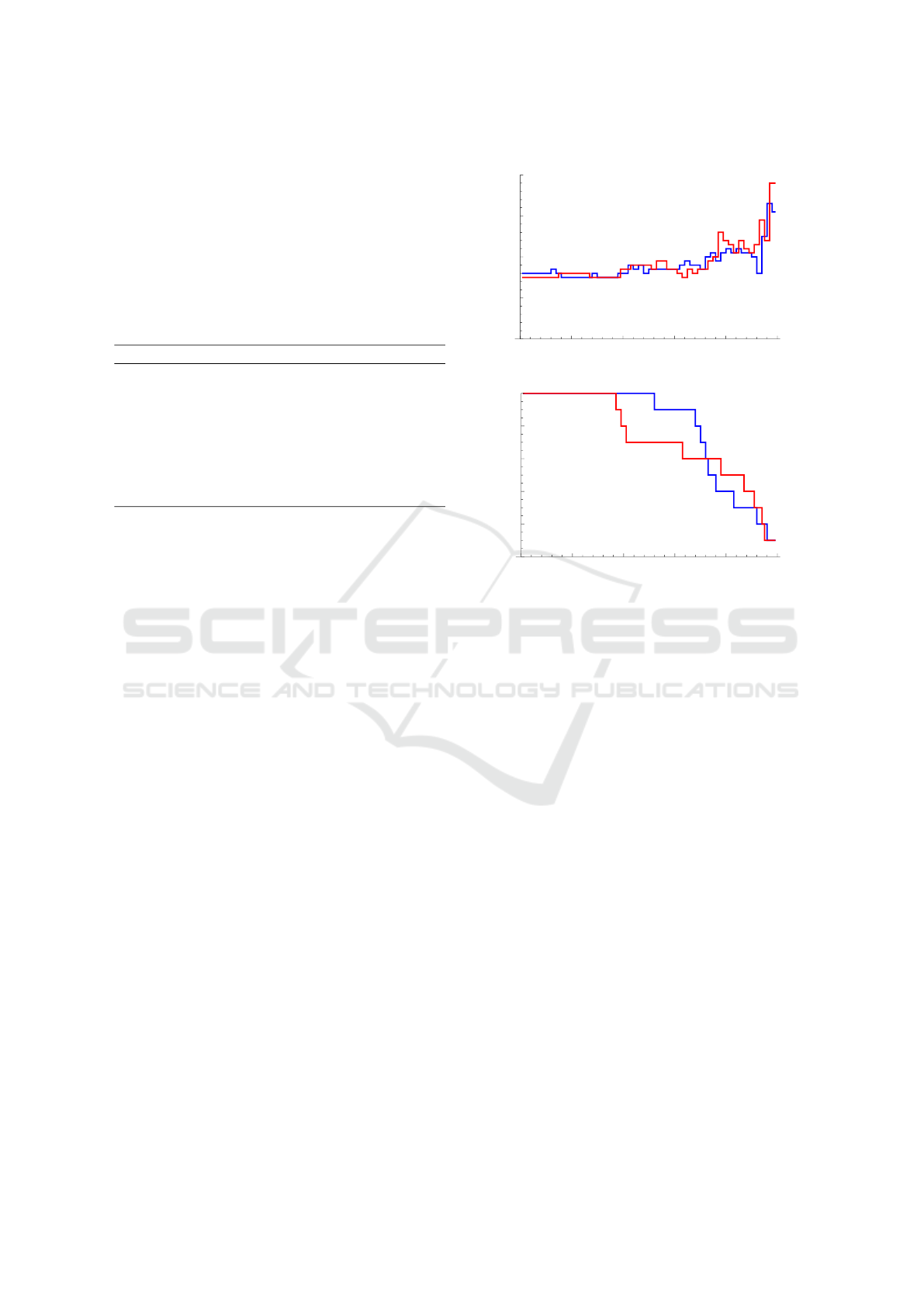
Figure 2 illustrates simulated sales processes in

the context of Example 3.1. Figure 2a illustrates price

trajectories of the two competing ﬁrms. Figure 2b

shows the associated evolutions of the inventory lev-

els. As demand is increasing in time, on average,

prices as well as the number of sales increase at the

end of the time horizon.

0 10 20 30 40 50

100

200

300

400

price

0 10 20 30 40 50

inventory

(2)

(1)

Figure 2: Simulated price paths (upper window 2a) and as-

sociated inventory levels over time (lower window 2b); Ex-

ample 3.1.

4 A HIDDEN MARKOV MODEL

WITH PARTIALLY

OBSERVABLE STATES

4.1 Theoretical Solution

In this section, we will assume that the competi-

tor’s inventory level cannot be observed. To derive

feedback pricing strategies we use a Hidden Markov

Model. We will use probability distributions for the

competitor’s inventory level, which are based on the

observable price paths of both ﬁrms.

Let π

(m) denote the (estimated) probability that

ﬁrm 2 has exactly m items left at time t; let ϖ

(n)

denote the probability that ﬁrm 1 has exactly n items

left at time t. We assume that the initial inventory

levels of both competitors are common knowledge;

i.e., the starting distributions are π

(m) = π

(m) =

{m=N

(2)

}

and ω

(n) = ω

(n) = 1

{n=N

(1)

}

. Further-

more, a run-out is observable, since we assume that

in case of a run-out a ﬁrm has to set its price equal to

zero. The evolutions of the probabilities π

(m) and

(n) are given by, n = 0, ..., N

(1)

, m = 0,...,N

(2)

, p

t−1+h

, p

t−1+h

∈ A, t = 0,1,...,T ,

Dynamic Pricing Strategies in a Finite Horizon Duopoly with Partial Information

t+h

(m;a

, p

) =

∑

, j

≥0,0≤m

−

≤N

(2)

m=(m

−

− j

)

(h)

, j

, p

) · π

−

)

(m;a

t−1+h

, p

t−1+h

) =

∑

, j

≥0,

0≤m

−

≤N

(2)

m=(m

−

− j

)

(1−h)

t−1+h

, j

t−1+h

, p

t−1+h

) · π

t−1+h

−

)

(12)

t+h

(n;a

, p

) =

∑

, j

≥0,0≤n

−

≤N

(1)

n=(n

−

−i

)

(h)

, j

, p

) · ϖ

−

)

(n;a

t−1+h

, p

t−1+h

) =

∑

, j

≥0,

0≤n

−

≤N

(1)

n=(n

−

−i

)

(1−h)

t−1+h

, j

t−1+h

, p

t−1+h

) · ϖ

t−1+h

−

(13)

Note, (12) and (13) are relevant for both ﬁrms as

they might try to estimate (i) the competitor’s inven-

tory level as well as (ii) the competitor’s beliefs con-

cerning the own inventory. This way the competitor’s

price reactions can be anticipated via a probability

distribution.

Both ﬁrms are assumed to act rationally. Pricing

decisions are such that no ﬁrm has an advantage to de-

viate from its strategy. Due to the deﬁned sequence of

events, theoretically, optimal decisions can be recur-

sively inferred. The corresponding value functions of

both ﬁrms, denoted by

(∗)

(n, p,

) (14)

(∗)

t+h

(m,a,

t+h

), (15)

are determined by the usual boundary conditions

(∗)

(0,·,·,·) = 0, V

(∗)

(·,·,·,·) = 0 (for ﬁrm 1)

and W

(∗)

t+h

(0,·,·,·) = 0, W

(∗)

T +h

(·,·,·,·) = 0 (for ﬁrm

2) as well as an associated system of Bellman

equations similar to (7)-(8) extended by transitions

for the beliefs, cf. (12)-(13). The correspond-

ing optimal feedback policies a

(∗)

(n, p,

) and

(∗)

t+h

(m,a,

t+h

) of the two competing ﬁrms can

be computed in recursive order (similar to (9)-(11)).

However, optimal policies cannot be computed in

practical applications. Note, the size of the state space

is exploding as the probability distributions

π and

are involved (curse of dimensionality). Hence, heuris-

tic solutions are needed.

In the following subsection, we present an ap-

proach to compute viable heuristic feedback pric-

ing strategies for the model with partially observ-

able states. The key idea is to approximate the func-

tions V

(∗)

(n, p,

) and W

(∗)

t+h

(m,a,

t+h

) by

using weighted expressions of the value functions

∗

(n,m, p) and W

∗

(n,m,a) (of the model with full

knowledge) and their associated policies a

∗

(n,m, p)

and p

∗

(n,m,a) derived in Section 3.

4.2 Solution with Partial Knowledge

Motivated by the Hidden Markov Model (HMM),

cf. Section 4.1, in which the competitor’s inventory

level cannot be observed, next, we want to deﬁne vi-

able heuristic pricing strategies for the two competing

ﬁrms. Based on current beliefs, we approximate the

correct value functions (14) - (15) (and related con-

trols) using price reactions (9) - (10) and future proﬁts

(7) - (8) of the fully observable model. As the value

functions of the fully observable model might system-

atically overestimate the correct values (14) - (15), we

include an additional positive penalty factor z. If z is

smaller than 1, future proﬁts (7) - (8) are reduced.

For ﬁrm 1 we deﬁne the feedback prices, t =

0,1,...,T − 1, n = 1, ..., N

(1)

, p ∈ A,

˜a

(n, p;

) = argmax

a∈A

(

∑

, j

≥0

(h)

, j

,a, p)

∑

0≤ ˜m≤N

(2)

( ˜m) ·

∑

0≤ ˜n≤N

(1)

( ˜n) ·

∑

, j

≥0

(1−h)

t+h

, j

{ ˜n−i

>0}

· a, p

∗

t+h



( ˜n − i

)

,( ˜m − j

)

{ ˜n−i

>0}

· a





(a − c

(1)

) · min(n,i

+ i

) + δ · z

·V

∗

t+1



(n − i

− i

)

,( ˜m − j

− j

)

{ ˜m− j

− j

>0}

·p

∗

t+h



( ˜n − i

)

,( ˜m − j

)

{ ˜n−i

>0}

· a



. (16)

Note, (16) mirrors the beliefs for both inventory

levels and the corresponding transitions. For antici-

pated price reactions we use p

∗

, cf. (10). To estimate

future proﬁts we use z ·V

∗

, cf. (7).

Similarly, the prices of ﬁrm 2 are given by, t =

0,1,...,T − 1, m = 1, ..., N

(2)

, a ∈ A,

ICORES 2018 - 7th International Conference on Operations Research and Enterprise Systems

˜p

t+h

(m,a;

) = argmax

p∈A

(

∑

, j

≥0

(1−h)

t+h

, j

,a, p)

∑

0≤ ˜m≤N

(2)

t+h

( ˜m) ·

∑

0≤ ˜n≤N

(1)

t+h

( ˜n) ·

∑

, j

≥0

(h)

t+1

, j

∗

t+1



( ˜n − i

)

,( ˜m − j

)

{ ˜m− j

>0}

· p



{ ˜m− j

>0}

· p





(p − c

(2)

) · min(m, j

+ j

) + δ · z

·W

∗

t+1+h



( ˜n − i

− i

)

,(m − j

− j

)

{ ˜n−i

−i

>0}

·a

∗

t+1



( ˜n − i

)

,( ˜m − j

)

{ ˜m− j

>0}

· p



. (17)

In each period, realized sales are used to update

the beliefs π and ω such that the prices (16) and (17)

can be computed during the sales process, i.e.:

˜a

(1)

,0;

)→

→ ˜p

(2)

;

)

→

→ ˜a

(1)

, p

;

)→ ...

... ˜a

T −1

(1)

T −1

, p

T −1

;

T −1

)→

T −1+h

→ ˜p

T −1+h

(2)

T −1+h

;

T −1+h

). (18)

Using simulations both ﬁrms’ expected proﬁts as

well as their distributions can be easily approximated.

Evaluating different z values makes it possible to

identify the (mutual) best z value.

4.3 Numerical Example

To illustrate our approach, in this subsection, we

consider a numerical example.

Example 4.1. We assume the setting of Example 3.1.

Both ﬁrms use the heuristic Hidden Markov strate-

gies, cf. (16) - (18), for different parameter values z,

0.2 ≤ z ≤ 1.5.

We observe that z has an impact on the expected

proﬁts of both competing ﬁrms. In our example, the

simulated average proﬁts of both ﬁrms are maximized

for z = 0.8. Note, the lower z is the more risk averse

(or aggressive) are the pricing policies (see standard

deviations σ), cf. Table 3.

Table 3: Simulated expected proﬁts and its standard de-

viations of both ﬁrms for different z values, Example 4.1.

z EG

(1)

(2)

(1)

(2)

σ(G

(1)

) σ(G

(2)

)

0.2 1141 1104 0.00 0.00 209 188

0.5 1679 1701 0.44 0.42 249 258

0.6 1743 1741 0.70 0.57 320 283

0.7 1742 1756 0.89 0.79 351 338

0.8 1739 1770 1.15 0.90 397 359

0.9 1732 1753 1.19 1.29 393 420

1.0 1716 1748 1.43 1.40 419 426

1.1 1686 1740 1.72 1.39 452 417

1.2 1668 1715 1.90 1.59 456 427

1.5 1647 1639 2.07 2.31 454 470

Remark 4.1. (Parallelization.)

The computation of feedback policies and particu-

larly extensive simulation studies can become CPU-

intensive. Parallelization can be used to compute re-

sults more efﬁciently:

(i) Feedback prices for the same point in time can

run in parallel.

(ii) Simulations can be computed independent from

each other.

Figure 3 illustrates simulated sales processes in

the context of Example 4.1. Figure 3a illustrates price

trajectories of the two competing ﬁrms. Figure 3b

0 10 20 30 40 50

100

200

300

400

price

0 10 20 30 40 50

inventory

(2)

(1)

E[X

(1)

,ω ]

E[X

(2)

,π ]

Figure 3: Simulated price paths (upper window 3a) and as-

sociated (estimated) inventory levels over time (lower win-

dow 3b), z = 0.8; Example 4.1.

Dynamic Pricing Strategies in a Finite Horizon Duopoly with Partial Information

shows the associated evolutions of the inventory lev-

els and the (mutually) estimated inventory levels of

the competitor (dashed plots).

5 UNKNOWN STRATEGIES

In this section, we want to present another heuristic

approach to derive effective pricing strategies in com-

petitive markets with limited information. We assume

that the strategy of the competitor is completely un-

known.

Our key idea to deal with unknown price reactions

is to assume sticky prices. For ﬁrm 1, we deﬁne the

following value function, p ∈ A, n ≥ 1, t = 0,1,...,T −

(0, p) = 0,

(n, p) = 0,

(n, p) = max

a∈A

(

∑

, j

(h)

, j

,a, p)

∑

, j

(1−h)

t+h

, j

,a, p) ·



(a − c

(1)

) · min(n,i

+ i

)

+δ ·

t+1



(n − i

− i

)

, p



. (19)

The heuristic strategy ¯a

(n, p) – determined by the

arg max of (19) – only depends on t, n, and p. Sim-

ilarly, the corresponding pricing strategy ¯p

(m,a) of

ﬁrm 2 is determined by the arg max of, a ∈ A, m ≥ 1,

t = 0,1,...,T − 1,

t+h

(0,a) = 0,

T +h

(m,a) = 0,

t+h

(m,a) = max

p∈A

(

∑

, j

(1−h)

t+h

, j

,a, p)

∑

, j

(h)

t+1

, j

,a, p) ·



(p − c

(2)

) · min(m, j

+ j

)

+δ ·

t+1+h



(m − j

− j

)



. (20)

The advantage of this approach is that the

value function does not need to be computed for

all competitors’ prices p in advance. The value

function and the associated pricing policy can be

computed separately for single prices p (e.g., just

when they occur). If the competitor’s strategy is not

known (which is often the case) it is not possible to

anticipate potential price adjustments. This feedback

strategy is able to react immediately if a change of the

competitor’s price takes place. In such an event, the

value function (19) - (20) and the associated prices

have to be computed for the new state.

Remark 5.1. (Oligopoly Competition.)

Note, due to the curse of dimensionality, the strategies

derived in Section 3 and 4 are just applicable when the

number of competitors is small. The heuristic strategy

described above, however, can still be applied when

the number of competitors is large! In case of K com-

petitors, the state p in (19) just have to be replaced by

~p = (p

(1)

,..., p

(K)

), p

(k)

∈ A, k = 1,...,K.

0 10 20 30 40 50

100

200

300

400

price

0 10 20 30 40 50

inventory

(2)

(1)

Figure 4: Simulated price paths (upper window 4a) and as-

sociated inventory levels over time (lower window 4b); set-

ting of Example 3.1.

For the case that the competitor’s strategy is un-

known, Figure 4 illustrates simulated sales processes

based on the heuristic, cf. (19) - (20), in the context

of Example 3.1. Figure 4a illustrates price trajectories

of the two competing ﬁrms. We observe that ﬁrms ei-

ther raise the price or undercut the competitor’s price.

Figure 4b shows the corresponding inventory levels.

6 STRATEGY COMPARISON

In this section, we want to compare the outcome of

our different solution strategies which take advantage

of different kind of information.

If pricing strategies are allowed to use full infor-

mation, i.e., the own inventory level, the competitor’s

inventory, and the competitor’s price, then the opti-

mal expected proﬁts can be computed analytically, cf.

ICORES 2018 - 7th International Conference on Operations Research and Enterprise Systems

Section 3. In case the competitor’s inventory level is

not known, we presented an approach to compute vi-

able strategies via a Hidden Markov Model, cf. Sec-

tion 4. If the competitor’s inventory is not known and

his/her pricing strategy as well as his/her reaction time

is not known, we proposed an efﬁcient heuristic.

By S

, we denote the strategy derived in Section

3 (full knowledge). By S

, we denote the response

strategy derived in Section 4 (partial knowledge) with

z = 0.8. By S

, we denote the heuristic strategy,

cf. Section 5, in case that the competitor’s strategy

is unknown. Considering the setting of Example 3.1

and Example 4.1, the expected proﬁts of the different

symmetric strategy combinations are summarized in

Table 4.

Table 4: Expected proﬁts EG

(1)

(of ﬁrm 1) and EG

(2)

(of

ﬁrm 2), when ﬁrm 1 and ﬁrm 2 play different pairs of strate-

gies: S

(both use full knowledge), S

(both use partial

knowledge), S

(mutually unknown strategies), cf. Exam-

ple 3.1 - 4.1.

Case EG

(1)

(2)

(1)

(2)

σ(G

(1)

) σ(G

(2)

)

FK 1754 1769 1.51 1.51 467 469

PK 1739 1770 1.15 0.90 397 359

UK 1771 1768 0.78 0.47 329 312

In the three cases expected total proﬁts, expected

remaining inventory, and standard deviations of to-

tal proﬁts have been approximated using simulations.

Surprisingly, we observe that in all three scenarios

both ﬁrms can expect similar proﬁts. It turns out that

as long as information structure is symmetric, a lack

of information does not necessarily result in smaller

expected proﬁts.

The number of unsold items (cf. load factor), as

well as the variance of proﬁts, however, have signif-

icant differences. In case of fully observable states

vs. S

) the remaining inventory and the vari-

ance of proﬁts is comparably high. Both ﬁrms can

expect almost equal results. In the second case with

partially observable states (S

vs. S

) we observe

that the load factor of both ﬁrms is higher and the vari-

ation of proﬁts is much smaller. Since less informa-

tion is available the competition between both ﬁrms is

less intense.

In case of mutual unknown strategies (S

vs.

) we obtain a similar result. Furthermore, we can

assume that the heuristic S

strategy will yield ro-

bust results when played against various other strate-

gies. The other two strategies are optimized to play

against a speciﬁc strategy. Hence, they might perform

less well, when the competitor is playing a different

strategy. Moreover, the efﬁcient computation of our

heuristic S

allows for fast computation times, and

in turn a high price reaction frequency, which is also

a competitive advantage.

7 CONCLUSION

In e-commerce, it has become easier to observe and

adjust prices automatically. Consequently, there ex-

ists an increased demand for dynamic pricing. The

computation of suitable pricing strategies is highly

challenging as soon as strategic competitors are in-

volved and remaining inventory levels play a major

role. In this paper, we analyzed stochastic dynamic

ﬁnite horizon duopoly models characterized by price

responses in discrete time. We allow sales probabili-

ties to generally depend on time as well as the com-

petitors’ prices. Further, we are able to model differ-

ent reaction times.

We have considered three different types of infor-

mation structure. In the ﬁrst setting, we assume that

the inventory levels of the competing ﬁrms are mutu-

ally observable. We show that optimal price reaction

strategies – which are based on mutual price anticipa-

tions – can be derived using standard methods (e.g.,

backward induction). Examples are used to identify

structural properties of expected proﬁts and feedback

pricing strategies. Optimal prices are balancing two

effects: (i) slightly undercut the competitor’s price in

order to sell more items, and (ii) the use of high prices

in order to promote a competitor’s run-out and to act

as a monopolist for the rest of the time horizon.

In the second setting, we assume that the inven-

tory of the competitor is not observable. Based on

observable prices, we compute probability distribu-

tions (beliefs) for the number of items the competitor

might have left to sell. We propose a simpliﬁed Hid-

den Markov Model to be able to compute applicable

feedback pricing strategies. Our examples show that

the resulting expected proﬁts of both ﬁrms are similar

to those obtained in the model with full knowledge.

The variance of proﬁts and the average number of re-

maining items, however, is signiﬁcantly lower.

In the third setting, we assume that the competi-

tor’s strategy is completely unknown, i.e., competi-

tors cannot anticipate price responses. We propose

an efﬁcient decomposition approach to circumvent

the curse of dimensionality and demonstrate how to

compute powerful pricing strategies. We verify that

– when applied by both competitors – the heuristic

yields the same expected proﬁts as in the two other

settings, in which more information is available.

To this end, we have shown how to compute ap-

plicable reaction strategies for real-life scenarios with

different information structures. We ﬁnd that ex-

Dynamic Pricing Strategies in a Finite Horizon Duopoly with Partial Information

pected proﬁts are hardly affected by less information

as long as the information structure is symmetric.

REFERENCES

Adida, E., G. Perakis. 2010. Dynamic Pricing and Inven-

tory Control: Uncertainty and Competition. Opera-

tions Research 58 (2), 289–302.

Chen, M., Z.-L. Chen. 2015. Recent Developments in Dy-

namic Pricing Research: Multiple Products, Compe-

tition, and Limited Demand Information. Production

and Operations Management 24 (5), 704–731.

Chung, B. D., J. Li, T. Yao, C. Kwon, T. L. Friesz. 2012.

Demand Learning and Dynamic Pricing under Com-

petition in a State-Space Framework. IEEE Transac-

tions on Engineering Management 59 (2), 240–249.

Gallego, G., M. Hu 2014. Dynamic Pricing of Perishable

Assets under Competition. Management Science 60

(5), 1241–1259.

Gallego, G., R. Wang. 2014. Multi-Product Optimization

and Competition under the Nested Logit Model with

Product-Differentiated Price Sensitivities. Operations

Research 62 (2), 450–461.

Levin, Y., J. McGill, M. Nediak. 2009. Dynamic Pricing in

the Presence of Strategic Consumers and Oligopolistic

Competition. Operations Research 55, 32–46.

Liu, Q., D. Zhang. 2013. Dynamic Pricing Competition

with Strategic Customers under Vertical Product Dif-

ferentiation. Management Science 59 (1), 84–101.

Martinez-de-Albeniz, V., K. T. Talluri. 2011. Dynamic Price

Competition with Fixed Capacities. Management Sci-

ence 57 (6), 1078–1093.

Phillips, R. L. 2005. Pricing and Revenue Optimization.

Stanford University Press.

Schlosser, R., M. Boissier. 2017. Optimal Price Reaction

Strategies in the Presence of Active and Passive Com-

petitors. 6th International Conference on Operations

Research and Enterprise Systems (ICORES 2017),

47–56.

Serth, S., N. Podlesny, M. Bornstein, J. Latt, J. Lin-

demann, J. Selke, R. Schlosser, M. Boissier, and

M. Uﬂacker. 2017. An Interactive Platform to Sim-

ulate Dynamic Pricing Competition on Online Mar-

ketplaces. 21st IEEE International Enterprise Dis-

tributed Object Computing Conference, EDOC 2017.

Talluri, K. T., G. van Ryzin. 2004. The Theory and Practice

of Revenue Management. Kluver Academic Publish-

ers.

Tsai, W.-H., S.-J. Hung. 2009. Dynamic Pricing and Rev-

enue Management Process in Internet Retailing under

Uncertainty: An Integrated Real Options Approach.

Omega 37 (2-37), 471–481.

Wu, L.-L., D. Wu. 2015. Dynamic Pricing and Risk Analyt-

ics under Competition and Stochastic Reference Price

Effects. IEEE Transactions on Industrial Informatics

12 (3), 1282–1293.

Yang, J., Y. Xia. 2013. A Nonatomic-Game Approach to

Dynamic Pricing under Competition. Production and

Operations Management 22 (1), 88–103.

Yeoman, I., U. McMahon-Beattie. 2011. Revenue Man-

agement: A Practical Pricing Perspective. Palgrave

Macmillan.

APPENDIX

Table 5: List of variables and parameters.

t time / period

(k)

shipping costs of ﬁrm k, k = 1,2

(k)

random future proﬁts of ﬁrm k

(k)

initial number of sold items of ﬁrm k

(k)

random inventory level of ﬁrm k

δ discount factor

h reaction time

(h)

sales probability for (t,t + h)

A set of admissible prices

V value function of ﬁrm 1

W value function of ﬁrm 2

a offer price of ﬁrm 1

p offer price of ﬁrm 2

n inventory state of ﬁrm 1

m inventory state of ﬁrm 2

π(m) beliefs of ﬁrm 1

ω(n) beliefs of ﬁrm 2

∗

, p

∗

strategies (full knowledge)

˜a, ˜p strategies (partial knowledge)

¯a, ¯p strategies (no knowledge)

ICORES 2018 - 7th International Conference on Operations Research and Enterprise Systems