Long Range Optical Truck Tracking
Christian Winkens and Dietrich Paulus
University of Koblenz-Landau, Institute for Computational Visualistics, Universit¨atsstr. 1, 56070 Koblenz, Germany
Keywords:
Off-road Platooning, Optical Tracking, Kalman filter, Autonomous Vehicles.
Abstract:
Platooning applications require precise knowledge about position and orientation (pose) of the leading vehicle
especially in rough terrain. We present an optical solution for a robust pose estimation using artificial mark-
ers and a camera as the only sensor. Temporal coherence of image sequences is used in a Kalman filter to
obtain precise estimates. Furthermore based on the marker detections we utilize an adaptive model building
algorithm which learns a keypoint based representation of the leading vehicle at runtime. The model is contin-
uously updated and allows a markerless tracking of the vehicle for up to 70 meters even when driving at high
velocities. The system is designed for and tested in off-road scenarios. A pose evaluation is performed in a
simulation testbed.
1 INTRODUCTION AND
MOTIVATION
A basic requirement for an intelligent vehicle is the
ability to detect and track other vehicles on its path
in order to perform platooning, namely, the automatic
following of a preceding vehicle. Therefore the so
called visual object tracking is an important platoon-
ing and computer vision problem which needs to full-
fill realtime requirements. One of the main challenges
of such a tracking system is the handling of appear-
ance changes of the vehicle during platooning. Ap-
pearance changes can be caused varying illumination,
out-of-plane rotation and vehicle motion. Put simply,
the goal is to localize the target vehicle in a video se-
quence, given a bounding box that defines the object
in an initial frame. Long-term tracking algorithms
generally consist of three different modules: a tracker,
that estimates object motion, a detector, that local-
izes the object in the current frame and a learner that
updates the object/background model. A variety of
approaches have been proposed however they mostly
differ in the choice of the object representation, that
can include: object silhouette, geometric primitives,
points and more. Many proposed algorithms use key-
points for object representation where the main idea
is to break down the object into individual parts that
are easier to match to a descriptor database than a
complete representation of the object. The tracker is
initialized by taking the initial bounding box as the
source for positive samples and the surrounding as the
M
1
M
2
tracked vehicle
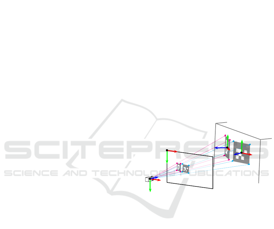
C
image plane
Figure 1: Imaging process P and measurements used for
pose estimation.
source for negative samples. One drawback of using
keypoints is that due to similar descriptors of object
and background elements matching is error-prone and
methods like RANSAC are needed to filter outliers.
The goal of our approach is to allow convoys to
move off-roads on rough terrain at relatively high ve-
locities, enabling precise position and orientation esti-
mation even with large distances between leading and
following vehicle. In order to solve these problem,
we use a mono-camera setup with a high image res-
olution and artificial markers on the leading vehicle
that allows an accurate pose reconstruction and makes
use of temporal coherence in order to track the lead-
ing vehicle with high precision in a short distance up
to 25 meters without any plane-world assumption as
proposed in (Winkens et al., 2015). Furthermore we
extend this approach and utilize a model learning al-
gorithm which uses the information from the marker
330
Winkens C. and Paulus D.
Long Range Optical Truck Tracking.
DOI: 10.5220/0006296003300339
In Proceedings of the 9th International Conference on Agents and Artificial Intelligence (ICAART 2017), pages 330-339
ISBN: 978-989-758-220-2
Copyright
c
2017 by SCITEPRESS – Science and Technology Publications, Lda. All rights reserved

reconstruction to initialize a keypoint based model
which is continuously updated and allows a marker-
less tracking of the vehicle for up to 70 meters even
when driving at high velocities or in rough terrain.
Our algorithm does not need any prior training or spe-
cial hardware for processing and relies only on artifi-
cial markers for initialization.
This work is structured as follows: Section 2 gives
an overview of related work and the pre-requisites for
the work presented. Our approach is then introduced
(Section 3)). An evaluation is presented in Section 4
and discussed in Section 5.
2 RELATED WORK
Several research topics have to be taken into account
when developing an extended pose estimation system
that utilizes marker-based and marker-less tracking
mechanisms. In the following paragraphs, the rele-
vant state-of-the-art techniques are briefly discussed.
2.1 Platooning
Platooning has already been discussed in many publi-
cations. Bergenheimet al. (Bergenhem et al., 2012)
provide a good overview to the topic. Vehicle-To-
Infrastructure Communication (V2I) or Vehicle-To-
Vehicle Communication (V2V) is utilized by a lot of
already published approaches such as (Gehring and
Fritz, 1997; Tank and Linnartz, 1997).
Benhimaneet al. (Benhimane et al., 2005) use a
camera and compute homographies to estimate the
pose of a leading vehicle. And Manzet al. (Manz
et al., 2011) utilize a particle filter, whereas
Frankeet al. (Franke et al., 1995) use triangulation.
2.2 Artificial Markers
Artificial markers are of common use, especially in
augmented reality (AR) and tracking applications.
Various different libraries have been developed and
are available free for use (Kato and Billinghurst,
1999; Schmalstieg et al., 2002; Fiala, 2005; Olson,
2011). We decided to use AprilTags (Olson, 2011) in
our system, to track a leading vehicle and to learn fea-
tures of it in an initialization phase. AprilTags allow
the full 6D localization of features from a single cam-
era image, which allows us a pose reconstruction of
an leading vehicle.
2.3 Tracking
The Kalman filter (Kalman, 1960) is of common use
in tracking applications. For example, Barth and
Franke (Barth and Franke, 2009; Barth and Franke,
2008) proposed a method for image-based tracking
of oncoming vehicles from a moving platform using
stereo-data and an extended Kalman filter. They used
images with a resolution of 640px by 480px.
Several surveys (Smeulders et al., 2014; Wu et al.,
2015) recently compared tracking performance of
several markerless trackers. According to the Vi-
sual Object Tracking challenge (VOT) (Kristan et al.,
2015; Kristan et al., 2016) challenge the top perform-
ing trackers applied learned features by convolutional
neural nets (CNN), which are quite new to the track-
ing community. The differences are found in differ-
ent localisation strategies. Due to the introduction of
neural networks huge progress have been made in re-
cent years. The MDNet tracker (Nam et al., 2014)
proposed by Nametal. is trained using a convolu-
tional neural network (CNN) and a set of videos with
ground-truth annotations to compute a generic repre-
sentation of the desired object. The winner of VOT
2016 (Nam et al., 2016) uses multiple collaborating
CNNs to track objects in visual sequences. Although
trackers based on neural networks deliver very good
results, they are mostly too slow, as the results of
(Kristan et al., 2015) indicate, to use them in realistic
tracking scenarios with real-time requirements right
now. Furthermore often special and costly GPUs are
needed for the algorithms to work. Usually it’s not
possible to train an object model a priori, the algo-
rithm must adapt to an object at runtime, which poses
a major drawback for CNN based methods which of-
ten rely on an a priori training.
Zhu et al. (Zhu et al., 2015) proposed an algo-
rithm which searches in the entire image for infor-
mative contours to adapt a generic edge-based object-
ness measure. Another method using kernel correla-
tion filters using the Fast Fourier Transform (FFT) is
presented by Henriquesetal. (Henriques et al., 2015),
which achieves good performance but cannot han-
dle the occlusion problem well. An real-time capa-
ble algorithm is presented by Henriqueset al. (Hare
et al., 2011), which extends an online structured out-
put SVM learning method, which is learned online,
to suit the tracking problem. Unfortunately Struck
does not handle scale variation, which is a major prob-
lem in our scenario where large scale variations ap-
pear. Another approach is to build models on the
distinction of the target against background by using
point features like BRISK (Leutenegger et al., 2011),
FREAK (Ortiz, 2012) or ORB (Rublee et al., 2011).
Long Range Optical Truck Tracking
331
Examples are proposed by Maresca et al. (Maresca
and Petrosino, 2013) and Nebehayetal. (Nebehay and
Pflugfelder, 2015). Nebehay uses BRISK features and
a static model in a combined matching and tracking
framework and a consensus-based clustering for out-
lier detection. Maresca however uses multiple key
point-based features together in combination with a
learning module which updates the object model, uti-
lizing a growing and pruning approach. Here the use
of multiple features sacrifices speed for improved ro-
bustness. As (Wu et al., 2015) stated, the use of a mo-
tion or a dynamic model is crucial for robust object
tracking, but the most evaluated trackers do not incor-
porate such components. Altough it could speed up
and improve robustness and efficiency. An active ap-
pearance model is used by Matthewset al. (Matthews
et al., 2004) to update models in an visual tracking
scenario.
3 OPTICAL TRACKING
APPROACH
In our setup we use a high resolution camera, which
is mounted on a vehicle that pursues a leading vehi-
cle. Two static artificial markers are mounted at the
back of the leading vehicle. This marker setup is ob-
served by the camera mounted on the following ve-
hicle. Obeserving the marker setup, our systems is
ablew to reconstruct the pose of the leading vehicle
at ranges up to 25 m and at the same time we learn a
model of the vehicle, so that a tracking of the vehi-
cle is possible when the markers can no longer recon-
structed because of a great distance from the preced-
ing vehicle. Furthermore, the learned model is used
to increase the stability of pose reconstruction done
by the Kalman filter in the close range.
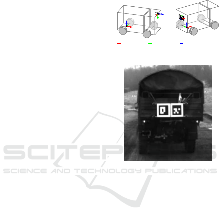
Figure 2 and Figure 3 illustrate the geometric
setup of the camera and the markers and define the
coordinate systems used in our system:
Symbol Coordinate System
C Camera
T Following Vehicle
M
i
Marker M
i
V Leading Vehicle
A pose is defined as the position and orientation
of an object in 3-D space. It is defined as a tuple
p = hs, qi with s ∈ IR
3
the position of the object rela-
tive to the origin of the coordinate system and q ∈ IR
4
the vector representation of a unit quaternion for the
rotation relative to the coordinate system’s orthonor-
mal bases.
T
C
M
i
V
x-direction
y-direction
z-direction
Figure 2: Defined coordinate systems and orientation of the
orthonormal bases.
Figure 3: Artificial marker mounted on leading vehicle.
Our system can deal with various marker setups
and configurations, but at least one marker is required
for our method to work. The precision of the pose
estimation will increase with higher numbers of (vis-
ible) markers.
In our setup, two artificial markers are mounted
on the back of the leading vehicle. They are slightly
rotated in order to be viewable from the side as well
(see Figure 3).
3.1 Kalman Filter
As the estimation of the pose of the leading vehicle
is prone to uncertainties, a Kalman filter (Kalman,
1960) is utilized to improve the pose estimate. The
dynamic Kalman state of the vehicle pose is repre-
sented by a vector:
x =
s
T
, q
T
, v
T
, ω
T
T
∈ IR
13
.
Where s = (s
x
, s
y
, s
z
)
T
the position and q ∈
IR
4
, q = (q
w
, q
x
, q
y
, q
z
)
T
, the vector representation of
a unit quaternion, define the position and orientation
ICAART 2017 - 9th International Conference on Agents and Artificial Intelligence
332
of the leading vehicle relative to the following vehi-
cle. The vectors v ∈ IR
3
and ω ∈ IR
3
describe the sys-
tem’s linear and angular velocity. For more details on
our kalman tracking system please refer to (Winkens
et al., 2015).
3.2 (Re-)Initialization
At first our system searches for our marker-system in
the given camera image. If visible the mounted mark-
ers are detected by our tracking system and a Kalman
filter is initialized. The pose of the leading vehicle
is tracked using the Kalman filter using a linear mo-
tion model. A good initial value of the pose p in the
dynamic state x is vital for proper estimation. When
launching the pose estimation process, pose p is ini-
tialized by solving the point correspondence problem
using the raw marker corner detections. If the algo-
rithm is not able to detect markers over a certain time,
it will fall back to the initialization mode.
3.3 Markerless Tracking
The maximum possible tracking range is directly lim-
ited by marker size and camera resolution. In order to
increase the range of the existing tracking system, it
is necessary not only to detect the markers and track
them, but to use the size of the vehicle and track the
vehicle itself. This requires to learn an abstracted
model of the vehicle, which is then used to track the
vehicle in each new frame of the data stream. As with
other trackers, the problem is then reduced to deter-
mine a bounding box enclosing the object, in each
frame. Our markerless tracking system is initialized
with the reconstructed pose and an initial bounding
box b
0
provided by the Kalman filter. The algorithm
then calculates keypointsκ
0
1
, ..., κ
0
l
on the initial frame
F
0
and splits them in object points K
0
= {κ
0
1
, ..., κ
0
l
}
and background points B
0
= {κ
0
1
, ..., κ
0
n
} by using the
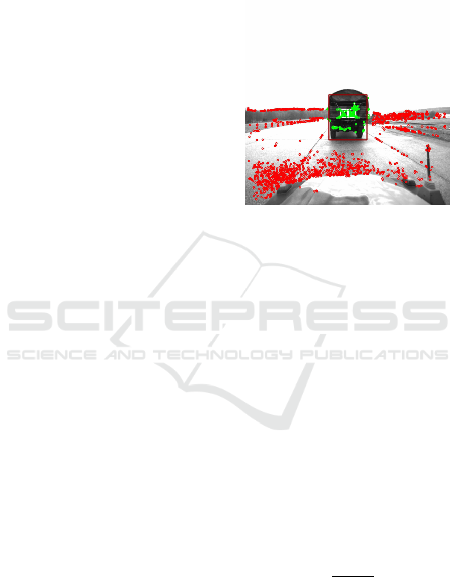
supported bounding box as illustrated in Figure 4.
Based on this bounding box we calculate ORB fea-
tures and store them in two separate models for each
element of the two sets of points. In addition, the cen-
ter of the bounding box and the pairwise distances be-
tween the feature locations is calculated and stored.
Furthermore, the object points are normalized by the
relative position of the feature points to the bound-
ing box center. After receiving the next frame F
t
the marker-based (Kalman filter) tracking first tries
to reconstruct a pose using the detected marker cor-
ners. In a second step the markerless tracking tries
to locate the desired object in the picture. A naive
approach would be to calculate the features through-
out the frame F
t
and search for correspondences with
Figure 4: Initialization of markerless tracker with K
0
as
nodel points (green) and B
0
as background points (red).
the object model. However, since the feature cal-
culation on a full resolution image would be very
time consuming the search space must be restricted
to meet real-time requirements. The initial object
model points are used to calculate the optical flow
(yves Bouguet, 2000) between the two frames:
κ
1
(x, y, t) = κ
1
(x+ dx, y + dy, 0 + dt) (1)
By utilizing optical flow a potential region of interest
can be estimated, which is expanded by a certain fac-
tor to account for uncertainties. This bounding box
defines a subregion F
p
t
of the frame, which is taken to
compute the features. The features {κ
t
1
, ..., κ
t
n
} ∈ F
t
are now matched against a model consisting of object
and background features. To prevent from false corre-
spondences between the model and candidates all fea-
tures that correlate with background features are di-
rectly discarded from the matching process. The rest
is matched utilizing the distance ratio method (Lowe,
2004) to filter false positives. The correspondences
thus found now give the set of ϒ
+
t
. After that the
matched correspondences using optical flow estima-
tion and global matching are fused, wherein the opti-
cal flow matches overrule the global matching. Using
the matched features we estimate scale s and rotation
α as proposed by (Kalal et al., 2010) and (Nebehay
and Pflugfelder, 2014).
s = med
(
||κ
t
i
− κ
t
j
||
||κ
0
i
− κ
0
j
||
, i 6= j
)!
(2)
α = med({atan(κ
0
i
−κ
0
j
)− atan(κ
t
i
−κ
t
j
), i 6= j}) (3)
A static appearance model is used, which is based
on the initial appearance of the object, composed of
Long Range Optical Truck Tracking
333

the initial descriptors K
0
. The model can not adapt to
appearance changes of the object or the background.
This is in the present scenario particularly relevant as
very large changes occur in the scaling of the object,
also the background can underly massive changes. To
account for this, the background model is adapted pe-
riodically to account for changes in the environment.
Features from the background database are picked
randomly and replaced by features from the current
frame, which do not intersect with the detected ob-
ject. Furthermore a homography is estimated based
on the matched features using the RANSAC method
(Fischler and Bolles, 1981). Correspondences which
do not correspond to the calculated homography are
sorted out as outliers. Thus, a correct data associa-
tion, which is essential for the reconstruction of the
points, can be achieved.
3.4 Feature Pose Reconstruction
Figure 5: Shematic description of our feature pose recon-
struction approach.
To support the marker based pose estimation, we
use features from the previouslylearned object model,
as described previously in 3.3. We try to estimate the
3-D position of these points, relative to the origin of
the preceding vehicle by accounting different obser-
vations of the feature in different frames during track-
ing, as illustrated by Figure 5. Knowing the 3-D po-
sition of the these feature points we could use their
observations in new frames to update the Kalman fil-
ter and support marker-based tracking.
The observation of a feature d
ij
which is seen from
camera pose c
i
can be expressed as an measurement
in the form:
h(m
j
, c
i
) = P (T (c
i
)
−1
· m
j
) (4)
Where P denotes the intrinsic camera model and
T (c
i
)
−1
describes the transformation of the feature
points in the coordinate system of the camera. Using
this prediction function the total back projection error
over alle features can now denoted as:
argmin
m
∗
,c
∗
∑
i
∑
j
||h(m
j
, c
i
) − d
ij
||
2
(5)
Which defines the sum of all differences between the
predicted h(., .) and the actually observed positions
of feature d
ij
. The minimum represents the opti-
mum utilization of all 3D feature positions and cam-
era poses. The optimization of this non-linear least-
squares problem is solved using the library Ceres
(Agarwal et al., ). The basic prerequisite for the bun-
dle adjustment described above is the robust tracking
of feature points from different camera views. Since
feature tracking is never perfect, the system must be
able to deal with outliers, or mistracked points. For
this reason, we use a robust loss function which lim-
its the influence of coarse outliers and effectively pre-
vents individualwrong tracked features from mislead-
ing the reconstruction.
Equation 5 is non-linear and non-convex. As a re-
sult, the convergence of the optimization process to
the correct solution strongly depends on initialization
parameters. We take the initialization of the camera
poses from the marker-based tracking and initialize
the feature locations in the origin of the preceding ve-
hicle. Simultaneously, a prior is set on the feature lo-
cations, which expresses a low certainty that the fea-
ture lies in the vicinity of the origin of the preceding
vehicle. This is useful to limit the uncertainty in z-
direction especially in the case of only a few observa-
tions with low baseline.
The used artificial markers are visible in nearly all
camera frames, which are used to reconstruct the fea-
tures and the corners of these markers can be seen as
normal feature points. But their position in the coor-
dinate system is fixed and known to our system, so we
use them to enhance the reconstruction because Ceres
allows selective fixing of parameters during optimiza-
tion. Therefore we add the corner points to the opti-
mization problem and declared them as fixed. The
fixed corner points also define the scale of the op-
timized points that could not be determined without
such a metric reference.
Solving this system of equations is computation-
ally intensive and requires much time. Each new
frame provides, according to the correspondences
found, new terms to the optimization problem, which
will bloat the system of equations in a short period of
time. Furthermore provide frames which are tempo-
rally close to each other little new information, since
the spatial distance between them is very low. Also
note that great distances between camera and vehicle
lead to worse results in feature matching and tracking.
Because the risk of false correspondencesheavily cor-
relates with increasing distance.
Therefore we ensure that only information from
camera poses with a euclidean distance of 0.2m and
more to the others is added to the system. In addition,
ICAART 2017 - 9th International Conference on Agents and Artificial Intelligence
334

only camera poses are added, which are below a dis-
tance of 20m to the vehicle driving ahead to minimize
risk of false correspondences.
Due to the automatic initialization of the mark-
erless tracking it is possible that features are used,
which do not belong to the vehicle or are very weak.
This may distract the tracking system in the long run
because it raises the chance of false correspondences.
Therefore, a model management has been integrated,
which periodically checks the quality of the model
and exchanges weak features. We calculate the re-
projection error of all reconstructed feature positions
with respect to all reconstructed poses and take the
mean. In a second step all features with an reprojec-
tion error greater than the mean are removed from the
model and new features are added instead.
3.5 Pose estimation
The learned and 3-D reconstructed model points are
additionally used by the Kalman filter at runtime to
improve the pose estimation. For this purpose, the
observations z
k
of the reconstructed keypoints m
j
are used as measurements for additional kalman up-
date steps. Observations are predicted similar to the
marker corner points using the measurement model:
ˆ
z
k
= P (T
T→C
· T
V→T
(p
k
, q
k
) · m
j
) + g
k
(6)
The two-dimensional random variable g
k
∼ N (0, R
k
)
models the measuring noise, which is assumed here
as 1px in the u- or v-direction.
The measurement model transforms the model
point m
j
using the p
k
, q
k
from the dynamic system
state x
k
of the Kalman filter into the coordinate sys-
tem of the following vehicle. Using the known po-
sition of the camera in the rear-running vehicle, the
point is transformed into the camera coordinate sys-
tem C. The function P performs a projection onto
the image plane as well as the radial distortion of the
point, just as before applying the known intrinsic cal-
ibration of the camera. The described Kalman update
step is executed exactly once for the model points ob-
served in the current frame. The remaining procedure
of the Kalman filter remains unchanged.
4 EVALUATION
The system is designed to work at high velocities
and in off-road scenarios. Therefore capturing ground
truth data for evaluation is a difficult issue, as a high
precision in the pose of both the following and the
leading vehicle is mandatory. External position track-
ing systems do not suit the demands as the required
off-road track is too long and it is therefore too cost-
and time-intense to equip with appropriate hardware.
Standaerd radio based position systems such as GPS
or Galileo do not offer an adequate pose quality.
Equipping one of the vehicles with hardware like 3-
D LIDAR sensors does not present a solution as well,
because the sensors themselves have uncertainties. To
make things worse, we consider an off-road scenario
where a full 6-D pose is required as a ground truth.
4.1 Evaluation using Synthetic Camera
Images
Our approach for evaluation of the marker-based
tracking is based on a virtual testbed. A simula-
tion environment is utilized for the generation of
synthetic camera images: The simulation environ-
ment used is derived from published approaches for
pose estimate evaluations (Fuchs et al., 2014b; Fuchs
et al., 2014a) using synthetic images. Its adaptive
architecture allows an easy integration. The camera
in the simulation environment can be configured to
match various resolutions and opening angles to test
the impact on the pose quality. The intrinsic cam-
era parameters needed for the pose tracking can eas-
ily be derived from the simulation configuration fol-
lowing the method described by Fuchsetal. (Fuchs
et al., 2014b). The evaluation results of our marker-
based tracking system were proposed previously in
(Winkens et al., 2015). A distance measurement de-
fined by Park (Park, 1995) was used and discussed by
Huynh (Huynh, 2009):
Γ(q, q
′
) = klog(Φ(q), Φ(q
′
)
T
)k
Where Φ : IR
4
→ IR
3×3
converts a quaternion to a ro-
tation matrix. In a first evaluation, the rendered image
sequences have directly been processed the Kalman
tracking as proposed above. In a second pass, Gaus-
sian noise N (0, I
2×2
) was added to the raw marker
detections extracted from the image. This way, we
were able to quantify the robustness of our method
using noisy data. The synthetic tests, as published
in (Winkens et al., 2015) show that the tracking sys-
tem has a translation error of 7, 3 cm at a distance of
8m.The average error in the orientation (avg|Γ|) is
0.06Rad ≈ 3.4Deg proving the robustness and preci-
sion of the system proposed.
4.2 Off-road Testing Scenario
Evaluation of the marker-free tracking extension for
long range outdoor tracking is difficult, as these syn-
thetic tests are not applicable. A good evaluation
Long Range Optical Truck Tracking
335
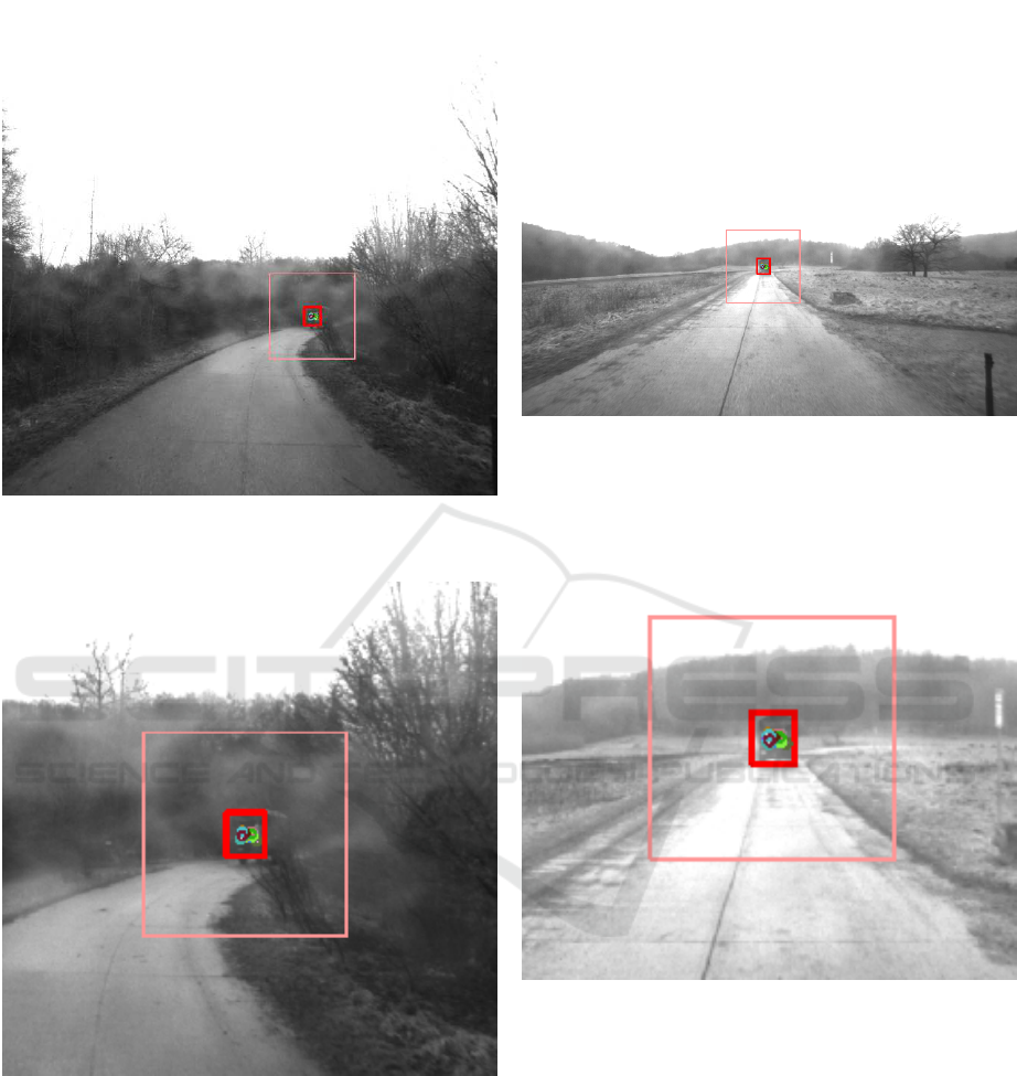
(a) Markerless tracking in the rain. The tracked vehicle is
marked with red bounding box.
(b) Magnified version, with tracked vehicle in red bounding-
box and matched features (colored circles).
Figure 6: Visualization of our long range markerless track-
ing during rain.
would require two Real Time Kinematic (RTK) sys-
tems mounted on both vehicles. Unfortunately, we
do not own such a system, but we plan to equip
our vehicles with it in the near future. Therefore
pose estimation system as proposed in this publication
has been tested and evaluated using datasets specif-
(a) Long range markerless tracking. The tracked vehicle is
marked with a red bounding box.
(b) Magnified version of the above image with matched fea-
tures from object model (colored circles).
Figure 7: Visualization of our long range markerless track-
ing.
ically recorded for this purpose with velocities up
to 60km/h. A truck with a artificial marker system
mounted on its back was followed by another vehicle
equipped with a high resolution camera. The recorded
data is used as the input for our system and is pro-
cessed in realtime. The vehicle tracked by our track-
ing system is highlighted with a red bounding-box in
the camera images, facilitating a visual examination
of our results in Figure 6 and Figure 7. Addition-
ICAART 2017 - 9th International Conference on Agents and Artificial Intelligence
336

ally we provide a video which can be viewed here
1
.
The examination showed that the system provided a
robust tracking up to a range of 70 m while process-
ing at 10 to 15Hz on standard mobile-computer hard-
ware. However, a quantitative analysis of the system
cannot be done in this scenario, because no reliable
ground truth pose information is available. Together
with this work we provide a video, which allows the
visual evaluation of the quality of the tracker.
5 CONCLUSION
We proposed an extended optical tracking mechanism
that only uses one camera and artificial markers to
track a vehicle driving at high velocities and great dis-
tances. A Kalman filter is utilized to include the ad-
vantages of temporal coherence. Our system is able
of estimating the relative pose between two vehicles
in real-time up to 26 m and tracking the vehicle itself
within a range up to 70 m. At an average distance of
8m, the average absolute of the Kalman filter error in
the translation, including artificial noise, (avg|∆|) is
about 7.3cm with an average error in the orientation
of(avg|Γ|) 0.06Rad ≈ 3.4Deg.
With the pose estimation and markerless track-
ing proposed, we introduced an algorithm capable of
tracking leading vehicles in off-road platooning sce-
narios, without the need for communication and/or in-
frastructure. The leading vehicle could therefore be a
regular truck equipped with a marker pattern. This
saves time and reduces costs significantly, as no com-
plex setup is necessary. The system works indepen-
dently from any external services and infrastructure.
The proposed system learns a model by detecting fea-
tures on the leading vehicle at runtime, so that the
pose of the vehicle can still be estimated even when
the leading vehicle gets too far away to detect the arti-
ficial markers. In closer range scenarios, dynamic fea-
tures improve the accuracy of the estimated pose. We
will further investigate the use of a second camera to
enhance tracking and pose estimation precision. Fur-
thermore we will equip our vehicles with some RTK
systems to provide a ground truth and allow a proper
evaluation in the near future.
ACKNOWLEDGEMENTS
This work was partially funded by Wehrtechnische
Dienststelle 41 (WTD), Koblenz, Germany.
1
https://www.dropbox.com/s/ly15h24085uyggp/
longrangetracking.mp4
REFERENCES
Agarwal, S., Mierle, K., and Others. Ceres solver.
Barth, A. and Franke, U. (2008). Where will the oncom-
ing vehicle be the next second? In IEEE Intelligent
Vehicles Symposium, pages 1068–1073.
Barth, A. and Franke, U. (2009). Estimating the driving
state of oncoming vehicles from a moving platform
using stereo vision. IEEE Transactions on Intelligent
Transportation Systems, 10(4):560–571.
Benhimane, S., Malis, E., Rives, P., and Azinheira, J.
(2005). Vision-based control for car platooning using
homography decomposition. In IEEE International
Conference on Robotics and Automation, pages 2161–
2166.
Bergenhem, C., Shladover, S., Coelingh, E., Englund, C.,
and Tsugawa, S. (2012). Overview of platooning sys-
tems. In Proceedings of the 19th ITS World Congress,
Vienna.
Fiala, M. (2005). Artag, a fiducial marker system using
digital techniques. In IEEE Computer Society Con-
ference on Computer Vision and Pattern Recognition,
volume 2, pages 590–596. IEEE.
Fischler, M. A. and Bolles, R. C. (1981). Random sample
consensus: a paradigm for model fitting with appli-
cations to image analysis and automated cartography.
Communications of the ACM, 24(6):381–395.
Franke, U., Bottiger, F., Zomotor, Z., and Seeberger, D.
(1995). Truck platooning in mixed traffic. In IEEE
Intelligent Vehicles Symposium, pages 1–6.
Fuchs, C., Eggert, S., Knopp, B., and Z¨obel, D. (2014a).
Pose detection in truck and trailer combinations for
advanced driver assistance systems. In IEEE Intelli-
gent Vehicles Symposium Proceedings, pages 1175–
1180. IEEE.
Fuchs, C., Z¨obel, D., and Paulus, D. (2014b). 3-d pose de-
tection for articulated vehicles. In 13th International
Conference on Intelligent Autonomous Systems (IAS).
Gehring, O.and Fritz,H. (1997). Practical results of a longi-
tudinal control concept for truck platooning with vehi-
cle to vehicle communication. In IEEE Conference on
Intelligent Transportation System (ITSC), pages 117–
122.
Hare, S., Saffari, A., and Torr, P. H. (2011). Struck: Struc-
tured output tracking with kernels. In Computer Vi-
sion (ICCV), 2011 IEEE International Conference on,
pages 263–270. IEEE.
Henriques, J. F., Caseiro, R., Martins, P., and Batista, J.
(2015). High-speed tracking with kernelized corre-
lation filters. Pattern Analysis and Machine Intelli-
gence, IEEE Transactions on, 37(3):583–596.
Huynh, D. (2009). Metrics for 3d rotations: Comparison
and analysis. Journal of Mathematical Imaging and
Vision, 35(2):155–164.
Kalal, Z., Mikolajczyk, K., and Matas, J. (2010). Forward-
backward error: Automatic detection of tracking fail-
ures. In In Proceedings of the 2010 20th International
Conference on Pattern Recognition, ICPR 10, pages
2756–2759. IEEE Computer Society.
Long Range Optical Truck Tracking
337

Kalman, R. E. (1960). A new approach to linear filtering
and prediction problems. Journal of Fluids Engineer-
ing, 82(1):35–45.
Kato, H. and Billinghurst, M. (1999). Marker tracking and
hmd calibration for a video-based augmented reality
conferencing system. In 2nd IEEE and ACM Inter-
national Workshop on Augmented Reality. (IWAR’99)
Proceedings., pages 85–94. IEEE.
Kristan, M., Leonardis, A., Matas, J., Felsberg, M.,
Pflugfelder, R.,
ˇ
Cehovin, L., Voj´ır, T., H¨ager, G.,
Lukeˇziˇc, A., Fern´andez, G., Gupta, A., Petrosino, A.,
Memarmoghadam, A., Garcia-Martin, A., Sol´ıs Mon-
tero, A., Vedaldi, A., Robinson, A., Ma, A. J., Var-
folomieiev, A., Alatan, A., Erdem, A., Ghanem, B.,
Liu, B., Han, B., Martinez, B., Chang, C.-M., Xu,
C., Sun, C., Kim, D., Chen, D., Du, D., Mishra, D.,
Yeung, D.-Y., Gundogdu, E., Erdem, E., Khan, F.,
Porikli, F., Zhao, F., Bunyak, F., Battistone, F., Zhu,
G., Roffo, G., Subrahmanyam, G. R. K. S., Bastos,
G., Seetharaman, G., Medeiros, H., Li, H., Qi, H.,
Bischof, H., Possegger, H., Lu, H., Lee, H., Nam, H.,
Chang, H. J., Drummond, I., Valmadre, J., Jeong, J.-c.,
Cho, J.-i., Lee, J.-Y., Zhu, J., Feng, J., Gao, J., Choi,
J. Y., Xiao, J., Kim, J.-W., Jeong, J., Henriques, J. F.,
Lang, J., Choi, J., Martinez, J. M., Xing, J., Gao, J.,
Palaniappan, K., Lebeda, K., Gao, K., Mikolajczyk,
K., Qin, L., Wang, L., Wen, L., Bertinetto, L., Ra-
puru, M. K., Poostchi, M., Maresca, M., Danelljan,
M., Mueller, M., Zhang, M., Arens, M., Valstar, M.,
Tang, M., Baek, M., Khan, M. H., Wang, N., Fan,
N., Al-Shakarji, N., Miksik, O., Akin, O., Moallem,
P., Senna, P., Torr, P. H. S., Yuen, P. C., Huang, Q.,
Martin-Nieto, R., Pelapur, R., Bowden, R., Lagani`ere,
R., Stolkin, R., Walsh, R., Krah, S. B., Li, S., Zhang,
S., Yao, S., Hadfield, S., Melzi, S., Lyu, S., Li, S.,
Becker, S., Golodetz, S., Kakanuru, S., Choi, S., Hu,
T., Mauthner, T., Zhang, T., Pridmore, T., Santopietro,
V., Hu, W., Li, W., H¨ubner, W., Lan, X., Wang, X.,
Li, X., Li, Y., Demiris, Y., Wang, Y., Qi, Y., Yuan,
Z., Cai, Z., Xu, Z., He, Z., and Chi, Z. (2016). The
Visual Object Tracking VOT2016 Challenge Results,
pages 777–823. Springer International Publishing.
Kristan, M., Matas, J., Leonardis, A., Felsberg, M.,
ˇ
Cehovin, L., Fernandez, G., Vojir, T., H¨ager, G.,
Nebehay, G., Pflugfelder, R., Gupta, A., Bibi, A.,
Lukeˇziˇc, A., Garcia-Martin, A., Saffari, A., Petrosino,
A., Montero, A. S., Varfolomieiev, A., Baskurt, A.,
Zhao, B., Ghanem, B., Martinez, B., Lee, B., Han,
B., Wang, C., Garcia, C., Zhang, C., Schmid, C., Tao,
D., Kim, D., Huang, D., Prokhorov, D., Du, D., Ye-
ung, D.-Y., Ribeiro, E., Khan, F. S., Porikli, F., Bun-
yak, F., Zhu, G., Seetharaman, G., Kieritz, H., Yau,
H. T., Li, H., Qi, H., Bischof, H., Possegger, H., Lee,
H., Nam, H., Bogun, I., chan Jeong, J., il Cho, J.,
Lee, J.-Y., Zhu, J., Shi, J., Li, J., Jia, J., Feng, J.,
Gao, J., Choi, J. Y., Kim, J.-W., Lang, J., Martinez,
J. M., Choi, J., Xing, J., Xue, K., Palaniappan, K.,
Lebeda, K., Alahari, K., Gao, K., Yun, K., Wong,
K. H., Luo, L., Ma, L., Ke, L., Wen, L., Bertinetto, L.,
Pootschi, M., Maresca, M., Danelljan, M., Wen, M.,
Zhang, M., Arens, M., Valstar, M., Tang, M., Chang,
M.-C., Khan, M. H., Fan, N., Wang, N., Miksik, O.,
Torr, P. H. S., Wang, Q., Martin-Nieto, R., Pelapur,
R., Bowden, R., Laganiere, R., Moujtahid, S., Hare,
S., Hadfield, S., Lyu, S., Li, S., Zhu, S.-C., Becker, S.,
Duffner, S., Hicks, S. L., Golodetz, S., Choi, S., Wu,
T., Mauthner, T., Pridmore, T., Hu, W., H¨ubner, W.,
Wang, X., Li, X., Shi, X., Zhao, X., Mei, X., Shizeng,
Y., Hua, Y., Li, Y., Lu, Y., Li, Y., Chen, Z., Huang, Z.,
Chen, Z., Zhang, Z., and He, Z. (2015). The visual
object tracking vot2015 challenge results.
Leutenegger, S., Chli, M., and Siegwart, R. Y. (2011).
Brisk: Binary robust invariant scalable keypoints. In
Proceedings of the 2011 International Conference on
Computer Vision, ICCV ’11, pages 2548–2555, Wash-
ington, DC, USA. IEEE Computer Society.
Lowe, D. G. (2004). Distinctive image features from scale-
invariant keypoints. International Journal of Com-
puter Vision, 60:91–110.
Manz, M., Luettel, T., von Hundelshausen, F., and Wuen-
sche, H.-J. (2011). Monocular model-based 3d vehi-
cle tracking for autonomous vehicles in unstructured
environment. In IEEE International Conference on
Robotics and Automation (ICRA), pages 2465–2471.
Maresca, M. E. and Petrosino, A. (2013). Image Analy-
sis and Processing – ICIAP 2013: 17th International
Conference, Naples, Italy, September 9-13, 2013, Pro-
ceedings, Part II, chapter MATRIOSKA: A Multi-
level Approach to Fast Tracking by Learning, pages
419–428. Springer Berlin Heidelberg, Berlin, Heidel-
berg.
Matthews, I., Ishikawa, T., and Baker, S. (2004). The tem-
plate update problem. IEEE Transactions on Pattern
Analysis & Machine Intelligence, (6):810–815.
Nam, H., Baek, M., and Han, B. (2016). Modeling and
propagating cnns in a tree structure for visual tracking.
arXiv preprint arXiv:1608.07242.
Nam, H., Hong, S., and Han, B. (2014). Online graph-based
tracking. In Computer Vision–ECCV 2014, pages
112–126. Springer.
Nebehay, G. and Pflugfelder, R. (2014). Consensus-based
matching and tracking of keypoints for object track-
ing. In Applications of Computer Vision (WACV),
2014 IEEE Winter Conference on, pages 862–869.
IEEE.
Nebehay, G. and Pflugfelder, R. (2015). Clustering of
Static-Adaptive correspondences for deformable ob-
ject tracking. In Computer Vision and Pattern Recog-
nition. IEEE.
Olson, E. (2011). AprilTag: A robust and flexible visual
fiducial system. In 2011 IEEE International Con-
ference on Robotics and Automation (ICRA), pages
3400–3407. IEEE.
Ortiz, R. (2012). Freak: Fast retina keypoint. In Proceed-
ings of the 2012 IEEE Conference on Computer Vision
and Pattern Recognition (CVPR), CVPR ’12, pages
510–517, Washington, DC, USA. IEEE Computer So-
ciety.
Park, F. C. (1995). Distance metrics on the rigid-body mo-
tions with applications to mechanism design. Journal
of Mechanical Design, 117(1):48–54.
Rublee, E., Rabaud, V., Konolige, K., and Bradski, G.
(2011). Orb: An efficient alternative to sift or surf. In
Proceedings of the 2011 International Conference on
ICAART 2017 - 9th International Conference on Agents and Artificial Intelligence
338

Computer Vision, ICCV ’11, pages 2564–2571, Wash-
ington, DC, USA. IEEE Computer Society.
Schmalstieg, D., Fuhrmann, A., Hesina, G., Szalav´ari, Z.,
Encarnac¸ao, L. M., Gervautz, M., and Purgathofer, W.
(2002). The Studierstube augmented reality project.
Presence: Teleoperators and Virtual Environments,
11(1):33–54.
Smeulders, A. W., Chu, D. M., Cucchiara, R., Calder-
ara, S., Dehghan, A., and Shah, M. (2014). Visual
tracking: An experimental survey. Pattern Analy-
sis and Machine Intelligence, IEEE Transactions on,
36(7):1442–1468.
Tank, T. and Linnartz, J.-P. (1997). Vehicle-to-vehicle com-
munications for avcs platooning. IEEE Transactions
on Vehicular Technology, 46(2):528–536.
Winkens, C., Fuchs, C., Neuhaus, F., and Paulus, D. (2015).
Optical truck tracking for autonomous platooning.
In Azzopardi, G. and Petkov, N., editors, Computer
Analysis of Images and Patterns: 16th International
Conference, CAIP 2015, Valletta, Malta, volume 9257
of LNCS, pages 38–48, Cham. Springer.
Wu, Y., Lim, J., and Yang, M.-H. (2015). Object track-
ing benchmark. Pattern Analysis and Machine Intelli-
gence, IEEE Transactions on, 37(9):1834–1848.
yves Bouguet, J. (2000). Pyramidal implementation of the
lucas kanade feature tracker. Intel Corporation, Mi-
croprocessor Research Labs.
Zhu, G., Porikli, F., and Li, H. (2015). Tracking randomly
moving objects on edge box proposals. arXiv preprint
arXiv:1507.08085.
Long Range Optical Truck Tracking
339
