
A CMOS Tracking System Approach for Cell Motility Assays
Cristina Martínez-Gómez
1,2
, Alberto Olmo
1,2
, Gloria Huertas
1,3
, Pablo Pérez
1,2
,
Andres Maldonado-Jacobi
1,3
and Alberto Yúfera
1,2
1
Instituto de Microelectrónica de Sevilla, CSIC- Universidad de Sevilla, Av. Americo Vespucio sn, 41092, Sevilla, Spain
2
Departmento de Tecnología Electrónica, ETSII, Universidad de Sevilla, Av. Reina Mercedes sn, 41010, Sevilla, Spain
3
Departamento de Electrónica y Electromagnetismo, F. Física, Universidad de Sevilla, Av. Reina Mercedes sn,
41010, Sevilla, Spain
Keywords: ECIS, Bioimpedance, Cell Culture, Cell Location, Cell Motility, Brownian Movement, CMOS.
Abstract: This work proposes a method for studying and monitoring in real-time a single cell on a 2D electrode
matrix, of great interest in cell motility assays and in the characterization of cancer cell metastasis. A CMOS
system proposal for cell location based on occupation maps data generated from Electrical Cell-substrate
Impedance Spectroscopy (ECIS) has been developed. From this cell model, obtained from experimental
assays data, an algorithm based on analysis of the 8 nearest neighbors has been implemented, allowing the
evaluation of the cell center of mass. The path followed by a cell, proposing a Brownian route, has been
simulated with the proposed algorithm. The presented results show the success of the approach, with
accuracy over 95% in the determination of any coordinate (x, y) from the expected center of mass.
1 INTRODUCTION
Cell motility plays an important role in many
biological processes, such as embryogenesis, wound
cicatrisation, immune response, and cancer evolution
(Ananthakrishnan, 2007). Tumour cell motility is
directly related with the processes of cancer
propagation, generating metastasis processes, which
is one of the main raison of death related with this
injury. The assays in-vitro of cell motility represents
a useful tool on the research on mechanism
regulation of the cancer cells migration, also to test
the efficiency of alternative drugs to combat cancer
at cellular level.
The most common methods for studying cell
motility are optics, based on microscopy, and with
fluorescence techniques. However, since these
methods are well established and referenced, they
require fluorescence markers, which can interfere on
correct function of some proteins, modifying the
normal cell evolution (Zhu, 2015). In addition, light
application at high intensity levels required for
exciting fluorescence compounds, can deliver or
generate some toxics elements at cells.
ECIS (Giaever and Keese, 1986) technique
allows cell culture research based on impedance
measurements done based on cell attachment
performance, to obtain cell properties, cell index,
etc. (Grimnes, 2008, Yeh, 2015). ECIS techniques
represent a non-invasive method for real time
monitoring of cells and definition of cell properties:
cell adhesion, motility, drug assays test, cell
growing, etc. (Sinclair 2012, Mondal, 2013).
Experimentally, ECIS technique requires of an
excitation signal, current (or voltage), applied to
obtain a voltage (or current) as response. The bio-
impedance information due to cell attachment to the
electrode is extracted from the signal response (real
and imaginary components, or magnitude and phase
(Mansor, 2015). The main problems to be solved for
extract this information are two. Firstly, bio-
impedance changes due to cell culture measurements
must be performed with accuracy using adequate
techniques and circuits with high performance
(Grimnes, 2008) (frequency programmable
voltage/current generators, amplifiers, demodulators,
etc). Secondly, data obtained for bio-impedance of
electrode-cell system should be decoded to rebuild
and find the information sought, in general, number
of cells in a culture.
The proposed system shown in Figure 1 can be
implemented in CMOS technology. It is composed
of a 2D matrix of electrodes, which act as “small
sensors” of bioimpedance (Yúfera, 2009), integrated
Martà nez-Gøsmez C., Olmo A., Huertas G., PÃl’rez P., Maldonado-Jacobi A. and YÞfera A.
A CMOS Tracking System Approach for Cell Motility Assays.
DOI: 10.5220/0006291502290236
In Proceedings of the 10th International Joint Conference on Biomedical Engineering Systems and Technologies (BIOSTEC 2017), pages 229-236
ISBN: 978-989-758-216-5
Copyright
c
2017 by SCITEPRESS – Science and Technology Publications, Lda. All rights reserved
229
on the same or similar silicon substrate that
employed by the CMOS circuits for measuring and
acquisition (Huertas, 2015). The circuits allow
row/file selection to drive the actual “pixel” under
test, and optimal frequency selection to optimize
sensor sensitivity and voltage applied to electrodes
.
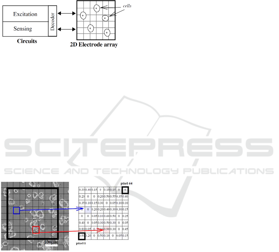
Figure 1: 2D electrode matrix and circuits for excitation
and acquisition electrical signals for biompedance test of a
cell culture.
The bio-impedance data obtained from cell
cultures can be employed to model the 2D system
proposed in Figure 1. In particular, it can be defined
the fill-factor parameter (ff) as the proportional area
filled by cell to the total area of one electrode. This
parameter oscillated from ff=0, when the electrode is
totally empty of cells (on top), to ff=1, if the
electrode is totally covered of cells. This system
gives us a dimensional matrix of numbers, one for
each pixel, in the range of 0 to 1, representative of a
cell culture status, as illustrated in Figure 2, for a
MCF7 cell line image, with an 8x8 electrode array.
In this way, black and white images can be created
from bio impedance measurements.
Figure 2: Fill-Factor map associated to each electrode, for
a MCF7 cell line image example.
The study proposed in this work focused on
spatial-temporal location of a single cell inside an
electrode matrix, using for that the information
obtained from sensors (pixels), in the form of ff map.
For that, it has been developed a Location Algorithm
implemented in Matlab. The proposed algorithm has
been applied to solve the problem to define the track
followed by a single cell in a culture, determining
the time evolution of its mass centre in a defined
period.
This document is organized as follows. Section 2
describes the proposed system structure and the
modelling of the cell under study. In section 3 it is
detailed how works the algorithm for locating a cell,
while section 4 describes its program
implementation, the simulations performed and the
validation process. Applications for a single cell
location and cell tracking will be shown. Finally,
section 5 will show the results obtained, and some
conclusions of the work, demonstrating the
correctness of the proposed algorithm to be applied
to study the metastasis problem.
2 SYSTEM MODELING
In this section, the proposed system structure to
develop the location algorithm is described. The first
step is addressed to model the cell which will be
used in the case study. There exists a wide variety of
cells with very different shapes and structures. For
the sake of simplicity, a circular cell is chosen in
such a way that it is defined by both the location of
the center of the circle (x, y) as well as the radio (r).
It should be taken into account that the circular cell
modelling is an ideal model and that elliptic
morphologies with variable radio could best
conform to the reality.
Once the shape and the size of the cell have been
specified, the second step is to define the
bidimensional array of electrodes. An array M of
NxN dimension, where each element M(i,j) includes
an electrode of fixed area, being i the position of the
row and j the position of the column. The array M
stores in each element its corresponding ff, generated
by the electrodes. These electrodes of the array are
considered squared and the side l.
To make easier the search algorithm and to
avoid, in advance, complex cases to be analysed,
when the cell is being located, the size of every
element of the array has taken equal or minor to the
cell diameter. The dimension of every element or
pixel (electrode) of the bidimensional array is equal
to the cellular diameter.
A series of concepts required during the
development of the system are defined below:
- Center of mass (cm): The center of mass of a
discrete masses system is a weighted average,
according to the individual mass, of the positions
of all the particles that compose it. It can be
calculated as:
BIODEVICES 2017 - 10th International Conference on Biomedical Electronics and Devices
230
∑
∑
1
(1)
M, the total mass of the particle system
m, the mass of the i-th particle
, position vector of the i-th mass with respect to
the assumed reference system.
- Relative error (): Is the quotient obtained by
dividing the absolute error and the exact value,
being the absolute error the difference between
the exact value and the measured value.
|
|
100
(2)
3 LOCATION ALGORITHM
The goal of the proposed algorithm is to obtain the
center of mass (cm) of the cell, for a given and fixed
occupation map, based on the ff or occupancy levels
of the different electrode array elements. With this
objective, an iterative algorithm has been developed
which assigns weights to each element of array
according to whether the 8 adjacent elements contain
occupancy values. In the algorithm, several elements
are defined:
The occupation array M above defined,
which includes the fill factor values. It
represents the data entry and is obtained
previously as a result of measurements made
on the system.
An empty subdivision array M
s
of 2Nx2N
dimensions, is also defined. It represents the
subdivision of the occupation array, where
each element M (i, j) is split into four. This
subdivision allows a more precise calculation
of which areas of each element are occupied
by the cell. In each iteration of the algorithm,
the M
s
array is subdivided into 4 sub-
elements and so on until an optimal result is
reached. The greater the number of divisions,
the more accurate the calculated center of
mass, but also the longer the required
runtime. This array stores the weights that
indicate which elements of it are parts of the
area of the cell under study (see Figure 3).
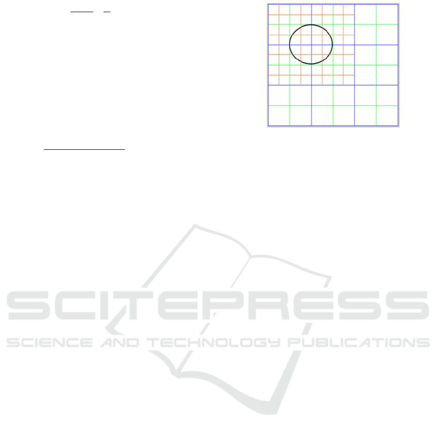
Figure 3: Array M of 3x3 dimension (blue), array M
s
of
6x6 dimension (green) and the subdivision of M
s
12x12
(red). The occupation map will have non-null values in the
two first elements of the two first rows. The subdivision
allows to calculate both which elements are part of the cell
and which are not and as a consequence obtaining its area
more precisely.
Taking the modeling references, the cell can
occupy a maximum of four elements of the
array M, i.e. there will be at most four non-
zero fill factors in the array. In this way, an
index vector I is defined that contains the
positions (i.j) of these four possible values of
M.
Array which stores the central points of
the greater weight elements of M
s
adjudicated
by the algorithm described later.
The algorithm can be divided into three
execution steps:
Step 1: Initialization: The occupation map
elements of M have input values given by the filling
factors resulting from the experiments. Firstly, an
initialization process is performed, according to
which the occupation map elements M are
subdivided into 4 sub-elements and the weights are
assigned, initializing the matrix Ms. These initial
values are selected according to the algorithm
proposed.
Step 2: Iteration: Secondly, the iterative process is
developed where the subdivision array, which
contains the weights, is subdivided into 4 sub-
elements and so on, at each iteration. At each level
of the iteration process, the current area resulting
from the algorithm is calculated. The process ends
when the areas obtained from the selected sub-
elements, for a determined level of iteration, are the
closest to the occupancy values obtained by the
sensors (ff).
A CMOS Tracking System Approach for Cell Motility Assays
231
Step 3: Calculation of the Mass Center: The
center of mass is calculated according to the results
obtained. From the resulting center of mass, the ff
s
corresponding to this point, called in the algorithm
ff
fb
, are calculated and compared with the real ff
s
of
the given occupation map. With this step, the system
is feedback in such a way that the mass center is
recalculated according to the difference obtained
between the calculated and actual ff, causing a
translation of the center of mass. This recalculation
process reduces the error in most of the cases.
The actions involved in each of the algorithm
steps are described below in a more detailed way:
Step 1.- Initialization
This step begins by traversing the M array,
which initially contains the values of the filling
factors resulting from biomedical experimentation.
The goal is to assign values to the subdivision array
M
s
.
Starting from each element M(i,j) with a non-
zero value and smaller than 0.75, weights are
assigned to the four sub-elements of the array M
s
which correspond to this element M(i,j). The
assigned weights are determinate by the values of
the 8 adjacent elements of M(i,j). In particular, the
weights will depend on:
If the neighbor of the diagonal contains a
non-zero value, then a constant A will be
added to the element M
s
adjacent to the
diagonal (see Figure 4).
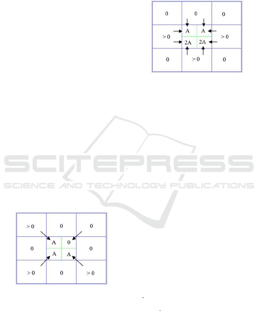
Figure 4: It despicts the diagonal adjacency of the central
element. For each adjacent neighbor of the diagonal of M
(blue), a weight A is assigned to the corresponding
element of the array M
s
(green).
If the remaining neighbors, which do not
conform the diagonal, contain a non-zero
value, then a constant A will be added to the
two elements of M
s
adjacent to the sides (see
Figure 5).
Figure 5: For each 4-adjacent neighbor of the array M
(blue), a constant value A is assigned to the two
corresponding elements of the array M
s
(green).
With this in mind, an element of M
s
will have at
most a weight of 3A.
On the other hand, if the value is higher than
0.75, the maximum weight, 3A, is straightaway
assigned to the 4 sub-elements (M
s
(2i-1,2j-1), M
s
(2i-
1,2j), M
s
(2i,2j-1), M
s
(2i,2j.
The array M is again examined and the following
conditions are established:
If 0
,
)
0.25, only the two larger
weight sub-elements of the four possible sub-
elements that would form M(i,j) are stored in
the array M
s
.
If 0.25
,
)
0.50, the three larger
weight sub-elements are stored in.
If
,
)
0.50, the four sub-elements of
M
s
are stored.
Step 2.- Iterative process
In this step the iterative process starts in order to
increase the resolution to obtain the area that most
closely matches the real area of the cell under study.
In each iteration the
array increases its dimension
as 2
numIter+1
N, being numIter, the iteration number in
which the process is and N the dimension of the M
array.
As in step 1, the M
s
array is examined and
weights are assigned to the new subdivision array,
M
s_iter
, according to the values of the adjacent
elements of M
s
. Calculating the weights of the new
array M
s_iter
elements, those that contain the
maximum weight with the same criteria established
in step 1 are selected. With these elements the
approached occupation area is calculated. As in each
iteration the subdivision increases, the area that
represents each element decreases and thus, the
BIODEVICES 2017 - 10th International Conference on Biomedical Electronics and Devices
232
percentage of occupation area of each element will
be given by:
4
(3)
At this point, the proposed by the algorithm
occupation area is evaluated, and compared to the
initial area, to which it must converge. If the
estimated by the algorithm area is equal to the
corresponding ff or approaches to a set range within
error margins, the iterative process is terminated.
Otherwise, step 2 is repeated to a maximum of 8
iterations. Once the iterative process is completed,
the geometric centers of the higher-weight elements
of the M
s_iter
array are stored in the array P. And in
turn, the mass center is calculated for each element
of index I, this calculation is based on the points P
contained within such elements. As discussed, there
will be a maximum of four ff values and therefore
four mass centers, calculated as follows:
1
,)
,,
,)
,,
(4)
where k defines the k-th value of the I vector and M
defines the total mass of the system, in our case, is
the sum of the ff whose value is always unitary.
Step 3.- Mass center of the cell calculation
The iterative process results in the four mass
centers related to each ff. With these points and
following the above equation, it is calculated the
mass center of the whole set corresponding to the
mass center of the cell.
(5)
To verify that the result is correct, our system is
feedback. The percentage of area occupied by the
obtained cell (ff
fb
) is calculated, and it is compared
with the original ff
s
. The fill factor and the mass
center of the cell are recalculated:
_
)
(6)
4 SOFTWARE
IMPLEMENTATION
The algorithm has been implemented in the
mathematical software tool Matlab. We divide this
section in two sections where different simulation
studies are carried out. First, in sub-section 4.1, an
example of the cellular localization based on the
localization algorithm is performed. Secondly, the
study and simulation of the cell trajectory described
in subsection 4.2 is implemented in Matlab.
4.1 Cellular Localization
In this section, an example of the operation and
results obtained with an array of 6x6 electrodes and
a 10μm diameter cell is shown. To properly simulate
the operation of cell cultures, the generation of the
position that the cell occupies on the surface of the
array is done in a random way. Once the mass center
is defined, the occupation map to be used by the
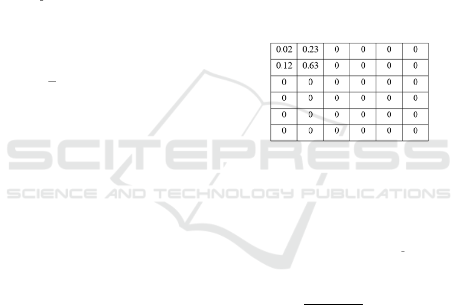
algorithm is calculated. Figure 6 shows an example
of the map obtained from a cell with center cm
real
(13µm, 48µm).
Figure 6: Occupation map of a cell with center in the
coordinates (x,y) = (13µm,48µm).
After five cycles of iteration, a set of points is
obtained, from which the center of the cell will be
calculated (Figure 7). Specifically two possible
centers are obtained, corresponding to the execution
of the algorithm without feedback (cm
cell
(12.63μm,
47.99μm)) and with feedback (cm
cell_fb
(12.87μm,
47.96μm)). The original cell is compared with the
two generated results and the relative error is
calculated with equation (7).
|
|
100
(7)
For the Y axis case both results are
approximated with an error lower than 0.05%.
However, for the X axis the error is reduced using
feedback (from 2.8% to a 1.0%). In Figure 8 it is
shown how calculated cells match real ones.
4.2 Cell Trajectory: Brownian Motion
The ECIS technique opens the possibility of
monitoring a cell culture in real time. In addition to
the estimation of the cellular location from a map of
A CMOS Tracking System Approach for Cell Motility Assays
233
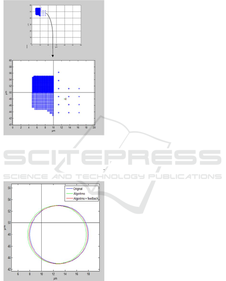
Figure 7: Resulting set of points for the elements with the
higher weight, corresponding to the elements of the
occupation map. In the selected part it is shown the real
centre cm
real
(13µm,48µm) (blue circle), the center
obtained with the algorithm cm
cell
(12.63µm,47.99µm)
(green line) and the center obtained with feedback cm
cell_fb
(12.87µm,47.96µm) (red line).
Figure 8: Comparison of the original cell (blue line) with
the calculated cell without feedback (green line) and the
calculated cell with feedback (red line).
occupation obtained with this technique, it is
interesting to have tools to analyze the temporal
evolution of the cell. In this way, the trajectories
described by them could be analyzed.
The mathematical modeling of cell movement is
of great relevance in the fields of biology and
medicine. Movement models can take many different
forms, but the most commonly used are based on the
extensions of simple random motion processes.
Assuming that motion is allowed in any direction,
this process is essentially known as Brownian motion
(Wu 2014, Qu, 2010). The physical phenomenon of
Brownian motion is based on the random motion of
particles suspended in a fluid as a result of their
collision with rapidly moving atoms or molecules.
To generate a two dimensional random motion,
two independent random paths are used, one for each
coordinate in time using different random seeds.
Instead of using random steps from a Gaussian
distribution, an approximation to Brownian motion
can be constructed by taking random measurements
of simple probability functions, such as a delta
function or a constant probability density function
(Codling 2018).
A Brownian motion model is implemented in
Matlab, indicating the starting point from which the
cell will start and the number of time samples desired
to obtain the points of the trajectory. Random angles
are generated for each moment and each mass center
is produced following a stochastic process:
)
1
)
cos)
)
1
)
sin)
(8)
In addition, the generation of the trajectory is
limited according to the size of the culture matrix.
Figure 9 and 10 show a possible trajectory
generated by the cell under study. After obtaining the
occupation map for each time instant, it is simulated
the trajectory followed using the localization
algorithm, previously implemented. To be specific, it
is considered a cell with an average velocity of 0.1
μm/min. The example simulates the calculation of
sixteen occupation maps for three hours.
As we checked in the previous point, most of the
points obtained with feedback are closer to the real
points. Table 1 shows for each point the errors
committed without feedback and with feedback, the
number of iterations made and the time used by the
system. The measurements have been obtained using
an Intel® Core ™ i7-4501U processor at 2.60GHz
and 11.9GB of RAM.
BIODEVICES 2017 - 10th International Conference on Biomedical Electronics and Devices
234
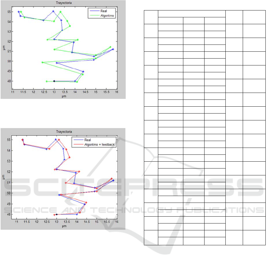
Figure 9: Real trajectory of a cell with radius 10µm (blue)
and trajectory calculated with the localization algorithm
(green).
Figure 10: Real trajectory of a cell with radius 10µm
(blue) and trajectory calculated with the localization
algorithm with feedback (red).
With these results we can verify that in most
cases the error decreases applying the feedback
process, being position 2 and 3 the only points where
the error is not improved. Even in these cases, errors
less than 3% are obtained. The majority of iterations
required to obtain the position is two cycles, reducing
the overall execution time of the trajectory. For
iterations less than 8 cycles the time spent is less than
60 seconds.
To confirm that the system developed in this
work is capable of robustly and accurately estimating
the position of the cell from the occupation maps, an
empirical study with more samples has been carried
out. These tests consist of the random generation a
cell track, with fifty points, each one with their
corresponding maps of occupation. The position
estimation of each of the cells generated applying the
Table 1: Error percentage for the 16 positions.
Pos
Relative error (
)
N_ite
CPU(s)
Axis x Axis y
1
Alg 2.85% 0.02%
5
56.70
Alg + fb 1.00% 0.08%
2
Alg 0.67% 0.14%
5
55.02
Alg + fb 1.12% 0.39%
3
Alg 0.12% 0,57%
8
70.50
Alg + fb 0.53% 0.33%
4
Alg 5.21% 0.06%
4
54.6
Alg + fb 0.64% 0.01%
5
Alg 0.74% 0.28%
2
54.01
Alg + fb 0.74% 0.01%
6
Alg 0.81% 0.46%
2
47.69
Alg + fb 0.49% 0.32%
7
Alg 0.67% 0.22%
2
47.90
Alg + fb 0.67% 0.06%
8
Alg 6.15% 0.51%
5
49.03
Alg + fb 2.95% 0.11%
9
Alg 1.34% 0.49%
2
48.21
Alg + fb 1.30% 0.24%
10
Alg 2.51% 0.14%
5
57.25
Alg + fb 0.70% 0.02%
11
Alg 2.76% 0.79%
2
48.14
Alg + fb 1.90% 0.41%
12
Alg 2.19% 0.16%
2
48.01
Alg + fb 1.07% 0.06%
13
Alg 2.68% 0.05%
4
51.4
Alg + fb 1.15% 0.05%
14
Alg 4.04% 0.15%
2
49.27
Alg + fb 1.18% 0.05%
15
Alg 1.72% 0.29%
2
47.90
Alg + fb 0.16% 0.07%
16
Alg 0.90% 0%
2
47.68
Alg + fb 0.24% 0%
algorithm and finally, the definition of the position of
each point generated applying the algorithm and its
feedback.
The highest errors obtained were located when
the occupation map collects most of the area in a
single element, but with connected elements with a
very low value. In contrast, when the cell is more
evenly divided into several elements, the error is very
small. And in the event that the cell is entirely in one
element or divided exactly in two or four elements,
the error obtained is null. Table 2 shows the
maximum and minimum error percentages obtained,
and an estimation of the mean error value.
A CMOS Tracking System Approach for Cell Motility Assays
235
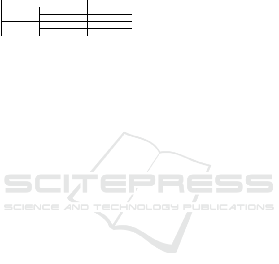
Table 2: Experimental error percentages.
Relative error () Max. Min. Mean
Algorithm Eje x 8.35% 0% 2.19%
Eje y 2.69% 0 % 0.49%
Algorithm +
Feedback
Eje x 4.98% 0 % 0.95%
Eje y 1.05% 0 % 0.19 %
With this experimental study, it is concluded that the
maximum error that the system can have is below
5% for the X axis and below 1% for the Y axis.
5 CONCLUSIONS AND FUTURE
WORK
A cellular localization system has been developed
based on the occupation maps generated by electrical
impedance spectroscopy. The localization system has
been able to generate the approximated cell position
in a culture, with a maximum relative error of 4.98%,
and a typical error of 1%, when it is provided
feedback to the algorithm. Although sometimes the
feedback does not reduce the error, in most cases
improves it, decreasing the error by half. The
proposed tracking algorithm enables CMOS
technologies for Lab-on-a-Chip systems for cell
motility assays, particularly useful in cancer research.
In order to expand the study, possible cellular
trajectories have been randomly generated following
the modeling of the Brownian system. Starting from
the trajectory it will be possible to perform studies on
the cellular behavior in different situations of interest,
as can be the effects of drugs in the cellular activity.
From the results obtained in this study, new lines
of research are opened that can be of great scientific
interest. Firstly, the cellular morphology is very
uneven and irregular, so the modeling of the cell in a
circular form does not resemble the reality, and
supposes an excessively simple model. A possible
improvement of the system would be to use modeling
of cells with more common form, for example, as an
ellipse. Tests with real cases can also be carried out,
using electrode arrays and a cell line of interest, to
characterize its trajectory and study its behavior.
Furthermore, variable side electrodes that do not
occupy the entire pixel could be used, and study, this
way, how to solve dead zones where no information
is collected and can be occupied by the cells.
ACKNOWLEDGEMENTS
This work was supported in part by the Spanish
founded Project: TEC2013-46242-C3-1-P: Integrated
Microsystem for Cell Culture Assays, co-financed
with FEDER.
REFERENCES
Ananthakrishnan, R., Ehrlicher, A., 2007. The Forces
Behind Cell Movement. Int J Biol Sci, vol. 3, n
o
. 5, pp.
303–317.
Zhu, Z., Frey O., et al., 2015. Time-lapse electrical
impedance spectroscopy for monitoring the cell cycle
of single immobilized S. pombe cells. Scientific
Reports, vol. 5, p. 17180.
Giaever, I. and Keese, C. R., 1991. Micromotion of
mammalian cells measured electrically, Proc. Nail.
Acad. Sci. USA. Cell Biology, vol. 88, pp: 7896-7900.
Grimnes, S., Martinsen, O., 2008. Bio-impedance and
Bioelectricity Basics, Academic Press, Elsevier, 2
nd
edition.
Yeh. C. F. et al., 2015. Towards an Endpoint Cell Motility
Assay by a Microfluidic Platform. IEEE Transactions
on NanoBioscience, vol. 14, n
o
. 8, pp. 835–840.
Sinclair, A. J. et. al, 2012. Bioimpedance analysis for the
characterization of breast cancer cells in suspension.
IEEE Trans Biomed Eng, vol. 59, n
o
. 8, pp. 2321–
2329.
Mondal, D., RoyChaudhuri, C., 2013. Extended electrical
model for impedance characterization of cultured
HeLa cells in non-confluent state using ECIS
electrodes. IEEE Trans Nanobioscience, vol. 12, n
o
. 3,
pp. 239–246.
Mansor, A. F. M., et al., 2015. Cytotoxicity studies of lung
cancer cells using impedance biosensor. In 2015
International Conference on Smart Sensors and
Application (ICSSA), pp. 1–6.
Huertas, G., Maldonado, A., Yúfera A., et al., 2015. The
Bio-Oscillator: A Circuit for Cell-Culture Assays.
IEEE Transactions on Circuits and Systems II, vol. 62,
n
o
. 2, pp. 164–168.
Yúfera, A., Rueda, A, 2009. A CMOS bio-impedance
measurement system. In 12
th
International Symposium
on Design and Diagnostics of Electronic Circuits
Systems, pp. 252–257.
Yúfera, A., Rueda, A., 2010. Design of a CMOS closed-
loop system with applications to bioimpedance
measurements. Microelectronics J. vol. 41, pp.231-
239.
Wu, P. H., et al, 2014. Three-dimensional cell
migrationdoes not follow a random walk. Proc
NatlAcad Sci U S A, vol. 111, n
o
. 11, pp. 3949–3954.
Codling E. A. et al., 2008. Random walk models in
biology. J R Soc Interface, vol. 5, n
o
. 25, pp. 813–834.
Qu B., Addison P. S., 2010. Modelling Flow Trajectories
Using Fractional Brownian Motion. In 2010
International Workshop on Chaos-Fractals Theories
and Applications (IWCFTA), pp. 420–424.
BIODEVICES 2017 - 10th International Conference on Biomedical Electronics and Devices
236
