Concept and Realization of a Diagnostic System for Smart Environments

Eric Heiden

, Sebastian Bader

and Thomas Kirste

University of Southern California, Los Angeles, U.S.A.

Institute of Computer Science, University of Rostock, Rostock, Germany

Keywords:

Automatic Diagnosis, Diagnostic Engine, Non-monotonic Reasoning, Model-based Diagnosis.

Abstract:

Automatically diagnosing a complex system containing heterogeneous hard- and software components is a

challenging task. To analyse the problem, we ﬁrst describe different scenarios a diagnostic engine might be

confronted with. Based on those scenarios, a concept and an implementation of a semi-automatic diagnostic

system are presented and some ﬁrst benchmarks are shown.

1 INTRODUCTION

Imagine you enter a smart conference room, connect

your laptop with the ﬁrst available HDMI-port and

the system automatically switches on the main pro-

jector. Smart Environments like this allow the user

to seamlessly interact with an ensemble of intercon-

nected devices. Sensors and actuators are combined

to provide an unobtrusive environment in which the

user’s intentions are inferred to facilitate multimedia-

enabled conferences or lectures. Immediately the ﬁrst

slide of your presentation appears on the screen and

you can start your talk. But suddenly the projected

display turns blank and you have to interrupt the pre-

sentation. What could possibly have happened? The

green power indicating LED of the projector is still

glowing and your laptop indicates it is duplicating its

screen via the HDMI connection, too. Perhaps the

display signal connection is broken? But after having

manually checked the ﬁrmness of every cable on the

way from your notebook to the projector the symptom

still persists. Finally you see no other option than ask-

ing the facility manager to look after the problem. A

short while later she ﬁnds the source of the error: the

projector’s lamp has exceeded its lifespan. Her expert

knowledge helped her diagnose the problem.

This contrived scenario gives rise to several ques-

tions: How could this situation be handled better?

What if we had expert knowledge immediately avail-

able without always having to seek out technicians to

identify and troubleshoot malfunctions? Which au-

tomatic methods do exist for the diagnosis of error

sources?

In this paper, we present an approach for a diag-

User

Knowledge

Diagnostic Engine

Middleware

System

description

Diagnosis

Observations

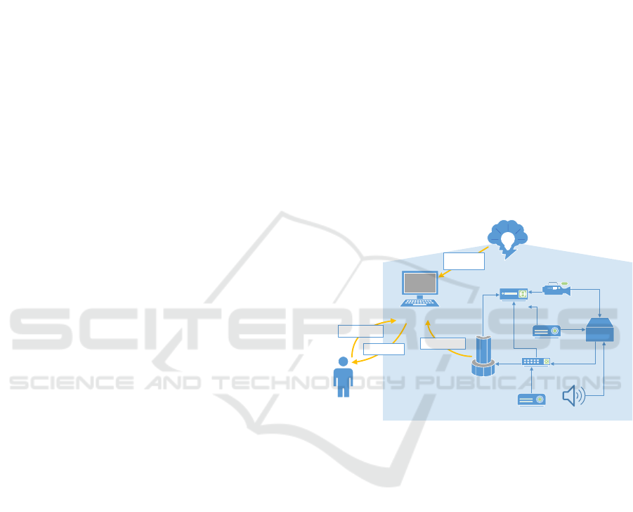
Figure 1: Context of the Diagnostic Engine.

nostic engine and its realization in our smart meet-

ing room. Figure 1 shows the context of a diagnos-

tic engine. The engine has predeﬁned knowledge of

the environment, i.e. the system of interconnected

components to be diagnosed. Provided with a symp-

tomatic observation, the engine reasons about possi-

ble sources of the encountered malfunction. To im-

prove these explanations, further observations can be

gathered using the middleware to retrieve status infor-

mation from the system’s components. As not every

detail is observable through the middleware, the en-

gine can also ask the user to provide observations.

First, we present a number of scenarios with in-

creasing difﬁculty in Section 2. We review different

approaches for diagnostic systems in Section 3. In

Section 4, we present our concept for a diagnostic en-

gine and describe our implementation in Section 5.

Finally, we present some preliminary benchmark-

results in Section 6.

318

Heiden E., Bader S. and Kirste T.

Concept and Realization of a Diagnostic System for Smart Environments.

DOI: 10.5220/0006257903180329

In Proceedings of the 9th International Conference on Agents and Artiﬁcial Intelligence (ICAART 2017), pages 318-329

ISBN: 978-989-758-220-2

2 DIAGNOSTIC SCENARIOS

In the following, several exemplary scenarios are de-

scribed to demonstrate different aspects of failure di-

agnosis. Scenarios are grouped by their difﬁculty from

a diagnostic engine’s perspective ranging from prob-

lems which can be detected by a single automatic

step, up to unsolvable issues which cannot be diag-

nosed, not even in cooperation with the user. The

analysis of problem classes furthermore allows to nar-

row down the diagnosis problem to only some sub-

systems which can be effectively treated by semi-

automatic diagnosis.

Scenarios are described by ﬁrst indicating what

the diagnostic engine knows about the system. This

a-priori knowledge consists of a wiring diagram rep-

resenting the system description, and the user’s ob-

servations on the state of the involved components. If

we are confronted with a diagnosis problem, these ob-

servations should contain symptomatic descriptions

which differ from the normal system behavior.

The omniscient perspective explains holistically

the actual system conﬁguration and true causes for

the occurring issues. If the diagnostic engine were

to know these facts, the proper diagnosis would be

calculable instantaneously. Subsequently, the partial

view of the system from the diagnostic engine’s per-

spective is examined to derive all possible diagnoses

the system can infer based on the observations and

its understanding of the system. If the diagnosis is

too vague to be useful for troubleshooting, the engine

makes further observations or asks the user to perform

these in order to gain more detailed information on the

true causes of symptoms.

These scenarios are contrived and are meant to fa-

cilitate a more lucid view on the general idea of di-

agnostic reasoning and probable pitfalls of automatic

diagnosing.

2.1 Automatically Identiﬁable Problems

This category contains scenarios which the diagnostic

engine can identify completely autonomously without

cooperating with the user, i.e. solely based on infor-

mation accessible through the middleware.

2.1.1 Complete Observations

The user tries to display content from laptop L on pro-

jector P but the screen remains blank. The user has

already observed that P is switched off and that all

involved devices and connections work as expected

without any problems.

Omniscient Perspective:

• All components work correctly.

• All involved cables are in proper condition.

• The projector is switched off.

Possible Error Sources:

• The projector is switched off.

This scenario represents the special case where the

provided observations are detailed enough to account

for a precise diagnosis. No further knowledge is re-

quired to infer that the powered off projector is the

single error source because it is given that all compo-

nents function.

2.1.2 Automatic Observations

The user tries to display content from laptop L on

projector P but the screen remains blank. L and the

control server S work as expected, and L provides an

HDMI video signal. All connections are stable. All

devices are switched on.

Omniscient Perspective:

• All components work correctly.

• All involved cables are in proper condition.

• S conﬁgured P to use the wrong input port.

Possible Error Sources:

• P is defect (e.g. projector lamp burned out, ﬁrmware

error, overheating, serious physical damage).

• S conﬁgured the wrong input on P.

• P ignores the conﬁguration carried out by S and hence

uses the wrong input.

The diagnostic engine is now confronted with an am-

biguous situation where multiple diagnosis candidates

compete. Here, a tie-breaking observation is neces-

sary. Let us assume that the engine asks S which in-

put conﬁguration has been set on P. S now requests

status information from P and reports P’s input con-

ﬁguration. This automatic observation reveals that P

is using the VGA port instead of HDMI to which L is

connected to. From this knowledge it can be inferred

that P is not defect (for simplicity we assume that if P

can be accessed via Ethernet it is completely ok) and

only S made the wrong input conﬁguration. Without

the need of human cooperation the engine could diag-

nose the symptom completely automatically. And the

system could subsequently ﬁx the problem automati-

cally by reconﬁguring P.

2.2 Semi-automatically Identiﬁable

Problems

Scenarios in which problems can only be diagnosed

in cooperation with the user belong to this category.

Concept and Realization of a Diagnostic System for Smart Environments

319

2.2.1 Non-automatically Observable System

Properties

Laptop L and projector P are switched on but P does

not show any output. The HDMI connection between

L and P is stable.

Omniscient Perspective:

• L works correctly.

• The HDMI connection between L and P is stable.

• The projector lamp in P has burned out.

Possible Error Sources: Let us assume that in this sce-

nario we have a more detailed model of projector P than

in the previous scenarios:

• P has a ﬁrmware bug.

• The projector lamp of P has burned out.

• The conﬁgured resolution of L is too high.

While the latter hypothesis can be discarded by per-

forming an automatic test if L’s resolution is greater

than the maximum resolution supported by P, the

ambiguity between the ﬁrst two diagnosis candidates

remains. In this case the user needs to check the

projector-related properties.

It can be argued that those two observations can

only be carried out by technicians and therefore the

true cause of error is still hard to retrieve. On the

other hand, the problem could be clearly limited to

projector P by the diagnostic engine so that in a real

world scenario the projector could just be replaced as

an immediate retaliatory action.

2.2.2 Multiple Simultaneous Faults

Both laptops, L

and L

, the server S and the projector

P are switched on and are in proper condition. How-

ever, P does not display anything.

Omniscient Perspective:

• All components work correctly.

• The HDMI cable between L

and P, and the VGA

cable between L

and P are broken.

• P is conﬁgured to use the VGA port as input source.

Possible Error Sources:

• The HDMI cable between L

and P is broken.

• The VGA cable between L

and P is broken.

• The HDMI cable between L

and P and the VGA ca-

ble between L

and P are broken.

First, the diagnostic engine should determine which

input has been selected by P. Therefore, S is commis-

sioned to request information on the input conﬁgura-

tion of P. This returns V GA as the active input port

and thus it can be reasoned that the VGA connection

between L

and P is broken.

Now that we are certain about one component of

our diagnosis it would also be helpful to know if there

might be any more faults in the system. Let us now

assume that P’s input conﬁguration is read-only so

that S cannot alter the setting automatically. How-

ever, in order to check whether the HDMI connection

between L

and P is broken, we need to test if P also

does not show anything if HDMI is selected as in-

put. Thus, the diagnostic engine has to ask the user to

carry out this diagnostic action and then tell whether

P shows something or not. The user reports that the

screen is still blank after HDMI has been deﬁned as

input. Ultimately, the diagnostic engine concludes

the following: both the HDMI connection between

and P as well as the HDMI connection between L

and P are broken.

If the user was unable to perform the diagnostic

step of altering the system’s conﬁguration to provide

a new observation, it would not be decidable whether

the HDMI connection between L

and P was broken

or not. A common approach to handle this knowl-

edge gap would be to assume that everything is work-

ing correctly unless we have concrete evidence to re-

tract such assumption (e.g. by observing a symptom).

Below we shall see how this type of so-called non-

monotonic reasoning is handled from a logical per-

spective.

2.2.3 Disconnected Subsystems

Until now, we have assumed that our diagnostic en-

gine somehow can instruct system-inherent compo-

nents, e.g. servers, to perform observations or alter

the system conﬁguration. In reality however, the di-

agnostician itself is a device or a software running on

network-attached hosts which might fail or loose con-

nection – just like any other component. To examine

this property in detail, let us assume the following sce-

nario: Laptop L, the diagnostic engine D und the NAS

(Network-Attached Storage) are connected to switch

S via Ethernet. While all devices are working as ex-

pected, L cannot connect to NAS.

Omniscient Perspective:

• All components work correctly.

• The Ethernet between D and S is broken.

• The Ethernet connection between NAS and S is bro-

ken.

Possible Error Sources:

• The Ethernet connections D – S and NAS – S are bro-

ken.

• The Ethernet connections D – S and L – S are broken.

• The Ethernet connections D – S, L – S and NAS – S

are broken.

The diagnostic engine cannot perform further obser-

vations automatically because it is disconnected from

the subsystem B = {NAS, L, S}. Therefore, all non-

empty permutations of broken Ethernet connections

between components c

, c

∈ B, together with the fact

that Ethernet connection D – S is broken, are valid

ICAART 2017 - 9th International Conference on Agents and Artiﬁcial Intelligence

320

diagnoses. This ambiguity can only be resolved if D

gets access to S or by asking the user to check all con-

nections.

2.3 Unidentiﬁable Problems

This class comprises diagnostic scenarios where the

diagnostic engine is unable to diagnose the symptoms

– not even in cooperation with a human user.

2.3.1 Hidden Interactions

After switching on a lamp, all lamps and projectors

are suddenly powered off.

Omniscient Perspective:

• All components work correctly.

• The lamps and projectors are connected to power

sources which share the same fuse.

• Due to power overload of too many connected de-

vices, this fuse was tripped and caused the power out-

age for all projectors and lamps.

Possible Error Sources: N/A

The engine cannot propose any diagnoses since it is

not aware of the interaction between projectors and

lamps. The fact that their power sources share the

same fuse might not be indicated in the wiring plan.

The engine cannot even ask the user to check the fuses

because it can only reason about facts which are pro-

vided as system knowledge.

Several approaches exist to handle hidden interac-

tions (see (B

ottcher, 1995; Kuhn and de Kleer, 2010)).

If we observe a malfunction which affects completely

unrelated parts of the system like in the given sce-

nario, it can be assumed that hidden, unintended in-

teractions have occurred.

2.3.2 Intermittent Abnormalities

In this scenario, the diagnostic engine runs directly on

the user’s laptop L.

The switch S intermittently becomes unavailable.

Laptop L is working correctly and the Ethernet con-

nection between L and S is stable.

Omniscient Perspective:

• Laptop L is working correctly.

• The Ethernet connection from L to S is stable.

• Switch S is congested sometimes when the user wants

to access it.

Possible Error Sources: N/A

Imagine that coincidentally, every time the diagnos-

tician tries to access S, the switch responds immedi-

ately. This observation contradicts with the user’s ob-

servation and in contrast shows no symptoms. There-

fore, it can only be reasoned that S is working cor-

rectly despite the apparent malfunction.

This problem could be addressed by letting the di-

agnostic engine constantly observe every network ac-

cess L is making. This kind of online diagnosis would

then experience – just like the user – the symptomatic

timeouts. However, during the course of this paper

only ofﬂine scenarios are considered in which a mal-

function has occurred and the user subsequently re-

quests an explanation of the observed symptoms.

2.3.3 Wrong Observations

Laptop L and projector P are switched on but P does

not show any output (cf. Scenario 2.1.1).

Omniscient Perspective:

• All components work correctly.

• The projector is conﬁgured to select its HDMI port as

input source.

• The observation provided by the user is wrong, i.e. P

indeed displays content from L.

Possible Error Sources:

• P is broken.

This diagnosis (that P is broken) is wrong because the

diagnostician trusted the user-provided observation

and does not have any automatic veriﬁcation methods

for given observations. Observations (human-made

or automatic) do not need to be invalid only because

of human deceit, often technical devices themselves

report false status information if they are broken, i.e.

they are behaving abnormally. This problem could be

tackled by assigning quantifying the degree of belief

when dealing with arbitrary inputs. A diagnostic the-

ory of involving probabilistic reasoning to deal with

uncertainty is given by (Lucas, 2001).

3 PRELIMINARIES

Before introducing two main concepts of diagnostic

reasoning, namely consistency-based and abductive

diagnosis, this section covers the general notion of di-

agnosis in the real-world context and its development

to an A.I. discipline.

While the term diagnosis can also mean the pure

decision whether a system is working or not, this pa-

per is based on the deﬁnition of diagnosis as a method

to identify the causes of observed system faults as pre-

cisely as possible.

Similar to real world diagnosis where experts are

asked to ﬁnd those parts in complex systems, like cars

or powerhouses, which account for the observed mal-

function, diagnosis as a subﬁeld in artiﬁcial intelli-

gence similarly provides techniques to identify causes

of observed symptoms – especially for applications

which require signiﬁcant expert knowledge. This task

Concept and Realization of a Diagnostic System for Smart Environments

321

requires observations of the actual, possibly unex-

pected system behavior as well as knowledge of the

problem domain sufﬁcient enough to infer meaning-

ful conclusions.

Diagnostic Engines ﬁrst emerged during the late

1960’s to early 1970’s in the form of rule-based ex-

pert systems (Angeli, 2010). Causal representations

of symptoms and faults were explicitly written as

hard-coded or compiled knowledge as an attempt to

mimic human expert behavior. These systems had

major drawbacks when applied to non-static domains

were properties evolve and affect the causal relation-

ships between observed problems and underlying er-

ror sources. Knowledge engineers were required to

cooperate with human experts in order to manually

update the knowledge base.

In contrast to these heuristic approaches, model-

based diagnosis which emerged during the 1980’s, al-

lowed for an estimation of system behavior which can

be compared to the observed outcomes in order to de-

tect abnormalities. These systems showed a higher

degree of robustness compared to rule-based systems

because they could better handle unexpected cases.

Current trends in diagnostic systems present the

coupling of classical model-based diagnosis with

other AI techniques like neural networks or genetic

algorithms (Angeli, 2010) to improve knowledge ac-

quisition and diagnose complex and dynamic systems

more effectively.

Model-based diagnosis is a commonly used

framework that works by modelling a system consist-

ing of interacting components or subsystems via log-

ical formulas. While it possible to deﬁne fault mod-

els, during the course of this paper only the system’s

expected behavior is modelled as in (Reiter, 1987;

de Kleer, 1986; Lucas, 2001). Conversely, the out-

puts of the real-world implementation of the system

are measured and the observations are as well logi-

cally formalized. The discrepancies between the ob-

servations and the predicted behavior are ﬁnally used

to diagnose faulty components whose behavior con-

tradict the model’s behavior.

Reiter proposed in (Reiter, 1980) a logic for de-

fault reasoning called default logic which extends

ﬁrst-order logic by allowing to perform default as-

sumptions. While in standard logic it can only be

stated that something is either TRUE or FALSE, de-

fault logic can express facts that are typically TRUE

only with a few exceptions.

For example, the fact that almost all projectors

have a VGA port can be represented as follows in de-

fault logic:

PROJECTOR(x) : M HAS-VGA(x)

HAS-VGA(x)

Here M stands for it is consistent to assume so that

this default rule can be read as: given the fact that x

is a projector (prerequisite) and it is consistent to be-

lieve that x has a VGA port (justiﬁcation), then one

may assume that x has a VGA port (conclusion). To

specify the notion of this consistency requirement, the

semantics of default logic is described in the follow-

ing.

A default theory is deﬁned as a pair (W, D), where

D is a set of default rules and W is the set of logical

formulas which deﬁne our background theory. If the

prerequisite of a given default D is entailed from our

theory W and every justiﬁcation is consistent with W

than we can add the conclusion to the theory.

Since the consequence relation is not monotonic,

default reasoning is a kind of non-monotonic reason-

ing.

First-order logic is monotonic, i.e. given two sets

A and B of ﬁrst-order formulas where A ` w, then

every model of A ∪ B is also a model of A so that

A ∪ B ` w. If we assume B to be newly discovered in-

formation, the addition of B to our existing knowledge

A does not affect the outcome w of A ∪ B with respect

to the models of A. That means, if later discoveries

reveal contradictions to formerly assumed rules they

cannot be retracted.

However, in any reasoning method were assump-

tions or beliefs are made, like default reasoning or

abductive reasoning (Section 3.2), it is necessary to

retract an assumption in order to avoid inconsisten-

cies with newly gained evidence. Adding knowledge

to the theory which contradicts the assumptions shall

invalidate them and thus reduce the set of conclu-

sions that can be derived from the theory. The notion

that further evidence does not monotonically grow the

set of derivable propositions describes the property of

non-monotonic reasoning.

3.1 Consistency-based Diagnosis

The theory by Reiter on Diagnosis from First Princi-

ples (Reiter, 1987) is a model-based approach which

conjectures about faulty components by only select-

ing hypotheses which are consistent with the sys-

tem’s model and the observations. This approach laid

an important foundation for the automatic identiﬁca-

tion of problems not only in electric circuitry as in

the early days of automatic diagnosis, but universally

across many different domains. In the following, di-

agnosis from ﬁrst principles will be used to present

the concept of consistency-based diagnosis.

In this model-based approach the only informa-

tion available to explain discrepancies between the

observed and correct system are ﬁrst principles, i.e.

ICAART 2017 - 9th International Conference on Agents and Artiﬁcial Intelligence

322

wor ks ( l ) :− n ot ab ( l ) .

wor ks ( p ) :− n ot ab ( p ) .

sh o ws ima ge ( p ) :− works ( l ) , works ( p ) ,

no t ab ( b ) , n ot ab ( hdmi ) .

Figure 2: Prolog implementation of a simple diagnosis ex-

ample.

the model of the system’s expected behavior repre-

sented using logical formulas. Reiter’s theory is ap-

plicable to any logic L which fulﬁlls the following

criteria:

1. Binary semantics so that every sentence of L has

value TRUE (>) or FALSE (⊥).

2. {∧, ∨, ¬} are supported logical operators which

have their usual semantics in L .

3.  denotes semantic entailment in L.

4. A sound, complete and decidable theorem prover

exists for L.

In general, ﬁrst-order logic (FOL) is only semide-

cidable, i.e. the question whether an arbitrary formula

f is logically valid (a theorem) in L can always be an-

swered correctly whereas a negative or no answer at

all will be given if f is not valid in L. To still fulﬁll the

last criterion, we will from now on deﬁne a decidable

subset of FOL as the logic L to be used for diagnosis.

This is established by requiring L to be a FOL with

ﬁnite domain of discourse D (Herbrand universe) and

ﬁnite Herbrand base.

Deﬁnition 1 (System). The system is deﬁned as a pair

(SD, COMPONENTS) consisting of SD, the system de-

scription which contains rules of logic L describing

the system’s normal behavior, and COMPONENTS, the

ﬁnite set of constants representing the components.

Components can be devices, connections, subsys-

tems, or any entity that could be (partially) respon-

sible for the system’s malfunction and should there-

fore be included in the diagnosis. The system descrip-

tion makes use of AB(c)-predicates which express for

component c ∈ COMPONENTS that c is behaving ”ab-

normally”. Thus, when modelling the intended sys-

tem behavior these abnormal-predicates only occur in

its negated form.

For a running example let us revisit our ﬁrst fully

automatically diagnosable scenario. In addition to the

system properties described before, let us also assume

that projector P’s lamp B is a component which can

burn out preventing P to show anything.

We could represent this scenario using the follow-

ing system description SDas a set of deﬁnite Horn

clauses shown in Figure 2 Similarly to SD, the obser-

vations are given as a ﬁnite set of logical formulas

in L as well. A diagnostic problem is deﬁned as the

triple (SD, COMPONENTS, OBS). For this example, let

OBS = {¬ IMAGE(P), WORKS(L)} be the set of our

observations, i.e. we observed that P did not show an

image and L was working.

A diagnosis for the problem

(SD, COMPONENTS, OBS) is deﬁned as the minimal

set (under set inclusion) ∆ ⊆ COMPONENTS where

SD ∪ OBS ∪ {AB(c) | c ∈ ∆} ∪ {¬AB(c) | c ∈

COMPONENTS\∆} is consistent.

Generally, a valid diagnosis would be the trivial

solution that all components are faulty, since we are

following the model-based approach were only the

expected behavior is known. Therefore, the Principle

of Parsimony has been established in (Reiter, 1987)

and advocates the minimal diagnosis. To ﬁnd minimal

diagnoses it helps to reformulate the aforementioned

deﬁnition of ∆ in terms of conﬂict sets.

A conﬂict set for (SD, COMPONENTS, OBS) is de-

ﬁned as C = {c

, . . . , c

} ⊆ COMPONENTS such that

SD ∪OBS ∪{¬AB(c

), . . . , ¬AB(c

)} is inconsistent. A

conﬂict set C is minimal iff no subset C

⊂ C exists

that is also a proper conﬂict set satisfying the equa-

tion.

Consistency-based diagnosis interprets the consis-

tency requirement by the semantics of classical logic

where a logical formula f ∈ L is consistent if f

has model, i.e. an interpretation or assignment of

variables of f to the domain of discourse D so that

the meaning of f is TRUE. Therefore, we can as-

sume the unresolved consistency terms WORKS(P)

and ¬WORKS(P) to be TRUE since a model exists

for SD ∪ OBS ∪ {AB(c) | c ∈ ∆} ∪ {¬AB(c) | c ∈

COMPONENTS\∆} ∪ {WORKS(P)} and another model

exists for SD ∪ OBS ∪ {AB(c) | c ∈ ∆} ∪ {¬AB(c) | c ∈

COMPONENTS\∆} ∪ {¬WORKS(P)}. As we will later

see, this consistency deﬁnition of non-stable models

marks the fundamental difference to abductive rea-

soning (cf. Section 3.2). The following two conﬂict

sets can be found:

= {AB(B), AB(P), AB(HDMI)}

= {AB(B), AB(L), AB(P), AB(HDMI)}

Hence we have the minimal conﬂict set is C

{AB(B), AB(P), AB(HDMI)}.

For a collection S of sets, a hitting set H for C is a

set H ⊆

S∈C

such that ∀S ∈ C : H ∩ S 6=

0. A hitting

set is minimal if no proper subset of it is a hitting set.

Reiter uses this deﬁnition to reformulate the charac-

terization of diagnoses: ∆ ⊆ COMPONENTS is a diagno-

sis for (SD, COMPONENTS, OBS) iff ∆ is a minimal hit-

ting set for the collection of minimal conﬂict sets for

(SD, COMPONENTS, OBS). For our example, three mini-

mal hitting sets can be found which represent our min-

imal diagnoses ∆

= {AB(B)}, ∆

= {AB(P)}, ∆

{AB(HDMI)}.

Concept and Realization of a Diagnostic System for Smart Environments

323

3.2 Abductive Diagnostic Reasoning

Abductive reasoning is a form of logical inferenc-

ing that hypothesizes explanations for a given ob-

servation, and is viewed as a competing concept to

consistency-based diagnosis. As a powerful concept

to handle commonsense reasoning, it has been applied

in the diagnosis domain (Eiter and Gottlob, 1995).

Abduction became a powerful reasoning method

to Artiﬁcial Intelligence especially in the ﬁeld of di-

agnosis which is considered by (Christiansen, 2005)

as one of the most representative and best understood

application domains for abductive reasoning. It has

further served as a basis for other types of expert sys-

tems, e.g. in the medical domain, and apart from di-

agnosis in areas such as planning, natural language

understanding and machine learning (Christiansen,

2005).

Abduction is a logical reasoning method that gen-

erates, given a logical theory or domain knowledge

T and a set of observations O, explanations (= hy-

potheses) E which explain O according to T such that

T ∪E  O, and T ∪E is consistent. Abductive reason-

ing is a type of non-monotonic reasoning since hy-

potheses E which have been made given theory T and

observations O might become obsolete due to new ob-

servations O

which require the reasoning system to

retract those explanations which do not meet the two

constraints from above. Therefore, default reasoning

can be based on abduction instead of non-monotonic

logics so that defaults are represented as hypotheses

to be made or retracted instead of deriving conclu-

sions within non-monotonic logics (cf. (Eshghi and

Kowalski, 1989)).

An abductive theory is a triple (P, IC, A), where

P is a logic program deﬁning the domain knowledge,

IC is a set of integrity constraints (logical formulas)

which deﬁne constraints on the abduced predicates,

and A is a set of abducible ground atoms.

We can now deﬁne express (P,IC, A) in terms of

the diagnosis domain in order to identify faulty com-

ponents ∆ ⊆ COMPONENTS in a malfunctioning system

in the same way as ﬁnding the best explanations for

given symptoms. A system (SD,COMPS) is formal-

ized as follows: SD is the system deﬁnition, as de-

ﬁned by P, and COMPS is the set of system components

which can be possible sources of errors, as deﬁned by

The integrity constraints IC can be used to ad-

ditionally constrain the generated diagnose, e.g. by

stating that certain components A

⊆ A cannot be di-

agnosed as faulty.

When diagnosing a system, one needs to observe

the malfunction and represent these symptomatic ob-

servations as a set of logical formulas OBS. The diag-

nosis problem (SD, COMPS, OBS) is solved through ab-

duction by retracting some of the ¬AB-assumptions.

The resulting set ∆ ⊆ A is a valid diagnosis if it ex-

plains all of the observed symptoms.

To meet the goal of providing useful diagnoses

which do not contain any, for the fault explanation

insigniﬁcant components, the Principle of Parsimony

advocates minimal diagnoses. Hence, a diagnosis

for (SD, COMPS, OBS) is according to (Ray and Kakas,

2006) a minimal set ∆ ⊆ A such that SD ∪∆  OBS∩IC.

We will use implementations of abductive reason-

ing in the form of logic programming and answer

set programming. These systems follow the stable

model semantics which was motivated by formalizing

the behavior of SLDNF resolution (selective, linear,

deﬁnite resolution with negation as failure), a com-

mon resolution strategy for logic programming sys-

tems like Prolog.

For any set M of atoms from Π, let Π

be the

program (reduct) generated from Π by removing

1. each rule that has a negative literal ¬l in its body

where l ∈ M, and

2. all negative literals in the bodies of the remaining

rules.

Since Π

is now negation-free, it has a unique mini-

mal Herbrand model. If this model is equal to M, then

M is a stable set of Π (Gelfond and Lifschitz, 1988).

Answer Set Programming (ASP) is a form of

declarative programming which is primarily ad-

dressed to solving NP-hard search problems. It has

its roots in Reiter’s theory of default reasoning and in

the generation of stable models.

In ASP, search problems are ﬁrst ground-

instantiated by so-called grounders like LPARSE

which are front-ends accepting logic programs. In

the next step, ASP solver like SMODELS or DLV

solve these computable search problems by calculat-

ing all stable models of the grounded programs. Un-

like SLDNF-employing reasoning tools like Prolog,

ASP solvers always terminate (Lifschitz, 2008). In

addition, the performance of current ASP solvers is

comparable to highly efﬁcient SAT solvers because

similar algorithms are used.

Consistency-based and abductive diagnosis both

represent techniques for identifying the error sources

of a malfunctioning system. Although these methods

can be applied to the same task, the results that are

calculated sometimes differ. In contrast, abductive di-

agnosis is more restrictive on the selection of diagnos-

tic explanations: the diagnosis ∆ in conjunction with

the system description SD must have a stable model

which logically entails the observations.

ICAART 2017 - 9th International Conference on Agents and Artiﬁcial Intelligence

324

One difference between consistency-based and

abductive diagnosis is that the former applies a

weaker criterion on valid diagnoses, because it uses

the consistency formula in the traditional FOL seman-

tic.

4 CONCEPT

The following section presents the conceptual ideas

and algorithm behind the implemented diagnostic en-

gine.

4.1 Reﬁning Hypotheses

The diagnosis ∆ is a set of hypotheses which ex-

plain the system’s malfunction based on the given

knowledge as logic program P and observations OBS.

Although can already calculate minimal diagnoses

which only select as few components as possible us-

ing consistency-based or abductive reasoning, there

are often too many explanations given to efﬁciently

isolate the true causes of the problem. In fact, model-

based diagnosis is often criticized for not being able

to ‘pinpoint a failing component from the available

symptom information’ (Koseki, 1989).

Therefore, further observations are necessary to

reﬁne the diagnosis. Let us assume that P is given

by the set of Horn clauses and our logic program sup-

ports negation as failure to be interpretable within sta-

ble model semantics.

What could be a further observation? Con-

sider our running example and its system description

shown as logic program in Figure 2. In the context

of semiautomatic diagnosis it is assumed that the user

does not know the true source of errors, i.e. faulty

components represented by AB-predicates. Based on

the observation of not shows

image(p) we can only

propose to observe works(l) or works(p) as these

two predicates belong to rules in P which further con-

tain AB-predicates. After the initial observation of

not shows image(p) the set of minimal diagnoses

would be {{l}, {p}, {b}, {hdmi}}. If the user would

observe works(l), then according to stable model se-

mantics the diagnostic engine would retract {l} from

the diagnosis. This reﬁnement of the diagnosis ex-

empliﬁes non-monotonic reasoning where additional

knowledge leads to the retraction of assumptions.

Starting from the initial, non-empty diagnosis ∆

which has been computed by at least a single obser-

vation of the system’s symptoms (otherwise ∆

since P is consistent) the diagnostic engine proposes

predicates G ⊆ P\(OBS ∪ {¬l | l ∈ OBS}) which have

not yet been observed (neither negated nor positive).

If the user or an automatic middleware system can ob-

serve the predicate p ∈ G, p or ¬p is added to our

observations OBS, depending on what was observed

about p. If p or ¬p are not observable, the diagnostic

engine should propose a new predicate for observa-

tion, if available. Otherwise, no more observations

can be proposed.

Algorithm 1 FINDABDUCIBLES(p, T, OBS) calcu-

lates the set of abducibles ⊆ ABDUCIBLES which can

be abduced from T ∪{p} in case p is observed. Here,

a reasoning system, e.g. ASP system is required in

order to calculate the stable models of the current the-

ory.

Algorithm 1: Finding abducibles.

procedure FINDABDUCIBLES(p, T, OBS)

R ←

// CSM = CalculateStableModels

for all A ← CSM(T ∪ OBS{p}, ABDUCIBLES) do

R ← R ∪ A

end for

return R

end procedure

Note that we are unifying the minimal diagnoses

which possibly consist of multiply components which

together must be faulty in order to explain the given

symptom. Instead of having sets of sets of possibly

faulty entities, the set representation of all candidates

allows us to quantify for each diagnosis step the utility

of an observation.

4.2 Proposing Observations

The information which abducibles can be eliminated

from the diagnosis ∆ if we observe that a predicate

p or its negation is true can then be used to propose

such p which maximally reduces ∆. Thanks to the Al-

gorithm 1 we can calculate which diagnosis (or any)

would result from observing p or ¬p so that we can

select a p which would result in the smallest possible

diagnosis 6=

4.3 Interactive Diagnosis

The diagnosis process as deﬁned in Algorithm 3 starts

with the knowledge base, i.e. program, P and a symp-

tomatic observation OBS which is a set of positive

or negated predicates occurring in P. The diagno-

sis ∆ is calculated by accumulating all abducibles

∈ A = {AB(. . . )} which explain the given observation

OBS. Using further, proposed observations as from

Algorithm 2, the diagnosis is reﬁned or assured: Ab-

ducibles contradicting ∆ will be used to reduce ∆ by

removing the negations of these abducibles.

Concept and Realization of a Diagnostic System for Smart Environments

325

Algorithm 2: Selecting the optimal observation.

Require: ∆ 6=

0 ∧ OBS 6=

0 ∧ ∆

⊂ ∆ ∧ ∀p ∈ P :

OBSERVINGCOST(p) > 0

procedure PROPOSEOBSERVATION(P, ∆, ∆

, OBS)

O ←

for all p ∈ P\(OBS ∪ {¬l | l ∈ OBS}) do

AB+

← FINDABDUCIBLES(p, P, OBS)

AB−

← FINDABDUCIBLES(¬p, P, OBS)

v ← min{p

AB+

, p

AB−

}

// if abducibles can be calculated.

O[p] ← v

end for

if O 6=

0 then

return argmin

p∈P\OBS

O[p]

else

return ⊥

end if

end procedure

Abducibles which conﬁrm ∆ will be added to the ﬁxed

diagnosis ∆

. ∆

is reﬂected during the diagnos-

tic reasoning process using the Integrity Constraints

IC. These constraints limit the calculated set of ab-

ducibles by only allowing abducibles which do not

conﬂict with ∆

. The diagnosis ﬁnishes if no further

observation can be proposed or if ∆ is small enough

so that the user can troubleshoot the problem.

5 IMPLEMENTATION

The implemented diagnostic system covers the full

workﬂow from extracting knowledge of semistruc-

tured wiring information to interactively providing

the user with diagnoses. This section ﬁrst covers the

general architecture of the implemented system and

then describes the necessary implementation steps in

detail from start to ﬁnish of the diagnosis workﬂow.

5.1 Architecture

The module for knowledge extraction takes as input

wiring information from a CSV (comma-separated

ProLogICA: abduce

dlv: diagnosis frontend

User

Diagnosis

Diagnostic Engine

Automatic observations as

additional LP Rules

Middleware

Logic Programming Rules

(Prolog, dlv)

Knowledge

Wiring information in CSV Empirical Knowledge

Device Mechanics

Device Interactions

Rules, facts, constraintsKnowledge

Diagnosis

sufficient or

empty

Calculate diagnosis

Observation

is automatable

Propose observation

yes

Observations

Observable property

Observations

Observable

property

yes

Knowledge Extraction

(Python)

Disjunctive Datalog

Abductive Logic Program

GraphViz

Figure 3: Architecture of the implemented Diagnostic Sys-

tem.

values) table and is further provided with device-

related code to model the behavior of different devices

as well as the interaction between them. This knowl-

edge can be represented via disjunctive datalog and

abductive logic programs. By formulizing the wiring

graph in DOT (a graph description language) it can

be visualized by graph drawing tools like dot or neato

from the Graphviz package.

Algorithm 3: The complete diagnosis process.

Require: P 6=

0 ∧ OBS 6=

Require: ABDUCE(G, P, IC, A) queries the Abductive Rea-

soner given the theory (P, IC, A) and goal G, and subse-

quently yields all minimal solutions ⊆ P (A) which ex-

plain G.

procedure DIAGNOSE(P, OBS)

∆ ←

∆

←

while (∆ not reﬁned enough and

∃p ∈ P : p 6∈ OBS and ¬p 6∈ OBS and

(({p} ∪ OBS ∪ P ∪∆

consistent) or

({¬p} ∪ OBS ∪ P ∪∆

consistent))) do

∆ ←

ABDUCE(OBS, P, ∆

, {AB(. . . )})

β ← PROPOSEOBSERVATION(P, ∆, ∆

, OBS)

if β = ⊥ then

return ∆

 No more observations can be proposed

end if

if β is observable then

AB+

, p

AB−

) ←

FINDABDUCIBLES(β, P, ∆, ∆

, OBS)

if β is observed as false then

OBS ← OBS ∪ {¬β}

∆ ← ∆\{¬l | l ∈ p

AB−

}

∆

← ∆

∪ p

AB−

else

OBS ← OBS ∪ {β}

∆ ← ∆\{¬l | l ∈ p

AB+

}

∆

← ∆

∪ p

AB+

end if

end while

return ∆

end procedure

The formal description as a logic program can then

be used via ProLogICA to ﬁnd diagnoses by perform-

ing abductive reasoning or DLV to diagnose using an-

swer set programming. The implemented Diagnostic

Engine uses DLV to generate diagnoses if provided

with an initial observation by the user. An interactive

loop has been implemented to reﬁne the calculated di-

agnosis based on automatic observations by querying

the middleware (e.g. publish-subscribe infrastructure)

or by instructing the user to conduct observations of

non-automatically observable system properties.

The interactive diagnosis session ﬁnishes once the

user accepts the diagnosis as reﬁned enough to trou-

ICAART 2017 - 9th International Conference on Agents and Artiﬁcial Intelligence

326

bleshoot the symptoms, or if there are no further ob-

servable (neither by a human nor the middleware) sys-

tem properties which could improve the diagnosis.

5.2 Knowledge Representation and

Reasoning

Diagnostic reasoning heavily depends on the provided

information of the implemented system and thus can

be seen as a discipline belonging to knowledge repre-

sentation and reasoning (KR).

The logical representation of a system and its di-

agnosis using logical reasoning has several advan-

tages over other diagnosis approaches:

• Logical formulae to describe the system structure

can be extracted easily from existing system data,

e.g. wiring diagrams or technical manuals.

• The logical rules are human-interpretable so the

user can comprehend and, if necessary, reproduce

the diagnostic reasoning.

• Only normal behavior needs to be modeled allow-

ing for smaller (human) effort to deﬁne the system

since no fault deﬁnitions are required.

• It is ensured that the calculated diagnosis is mini-

mal, i.e. the minimal set of possible sources of er-

ror is returned. This reduces further troubleshoot-

ing efforts.

Because of the pecularities of the two target plat-

forms, ProLogICA and DLV, two separate modules

have been implemented to formalize wiring informa-

tion as logic programs, namely Abductive Logic and

Datalog Programs. This decision was enforced for the

following reasons:

• ProLogICA relies on the non-declarative (linear)

semantic of python so that transitive connections

cannot be deﬁned recursively (in contrast to DLV)

conn(A,C) : −conn(A, B), conn(B,C).

but instead must be stated using a helping predi-

cate rconn which handles the recursion so that

rconn(A,C) : −conn(A, B), rconn(B,C).

• ProLogICA exhibits poor performance on too

many nested and especially non-grounded rules.

Thus, connections between all devices have been

resolved via depth-ﬁrst search.

• Not-AB-statements cannot be written as

not(ab(...)) but only not ab(...) in DLV while the

latter syntax was not supported on the used SWI

Prolog implementation.

• DLV requires AB-statements to be grounded,

while this leads to cryptic constants in Prolog.

5.3 Available Implementations

The diagnostic engine has been realized using two

different implementations: the answer set program-

ming environment DLV and the abductive reasoning

tool ProLogICA.

DLV stands for DataLog with Disjunction (where

V represents the logical operator ∨) and is a disjunc-

tive logic programming system. Rules can be written

in disjunctive datalog (function-free) of the form

∨ ·· ·∨ a

← b

, . . . , b

, ¬b

k+1

, . . . , ¬b

k+m

which allows DLV as an ASP system to solve prob-

lems whose complexity lies beyond the solvable

scope of non-disjunctive programming. DLV imposes

a safety condition on variables in rules such that a rule

is logically equivalent of its Herbrand instances.

DLV provides a diagnosis front-end for Abduc-

tive Diagnostic Reasoning as well as for Consistency-

Based Diagnosis. As described in (Eiter and Gottlob,

1995), a diagnostic problem represented by the set of

observations OBS, the system description SD and the

set of AB-atoms can be rewritten in disjunctive data-

log so that every stable model which the ASP solver

ﬁnds represents a diagnosis. The input programming

language for this front-end however does not support

disjunctive datalog and instead falls back to tradi-

tional datalog (function-free logic programming).

ProLogICA is an implementation of Abductive

Logic Programming (ALP) in Prolog. It allows the

user to deﬁne in a single ﬁle the abductive theory

(P, IC, A), where P represents the set of rules to de-

scribe the domain knowledge, IC is a set of integrity

constraints, and A declares the abducible predicates

(Ray and Kakas, 2006).

In contrast to competing implementations of ab-

ductive reasoning, ProLogICA allows the occurrence

of negated abducibles so that the formalization of nor-

mal system behavior can be made as described in Re-

iter’s Theory.

5.4 Semi-Automatic Diagnosis

Human-machine cooperation is realized via propos-

ing system properties to the user which would im-

prove the diagnosis. This section presents the im-

plementation of this fundamental aspect of semi-

automatic diagnosis.

Given a scenario as logic program which repre-

sents the system description, and a ﬁle of hypoth-

esis declarations which describe the possible AB-

predicates to be assumed as a diagnosis, the user ﬁrst

needs to provide an initial observation. Then, a di-

agnosis is calculated. If this calculation fails, the ob-

servations contain a contradiction or no hypotheses

Concept and Realization of a Diagnostic System for Smart Environments

327

−2

Number of abducible predicates

Time in seconds

FDsingle

FRsingle

FRmin

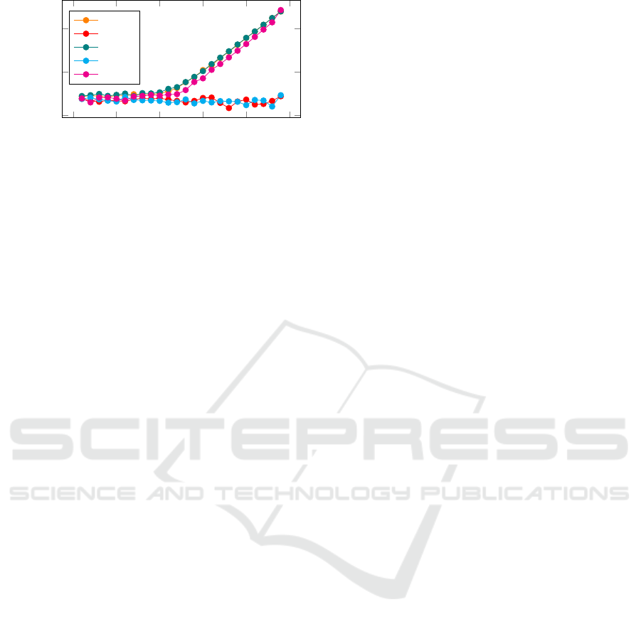
Figure 4: Benchmark Results of the DLV Diagnosis Fron-

tend.

could be found. In order to simulate automatic ob-

servations, an additional ﬁle can be provided which

contains non-abducible predicates either negated (us-

ing not) or non-negated. If the ranking of possible

observations returns predicates that are automatically

observable, these observations are added to the set of

current assumptions. If there are no automatic ob-

servations, the user is asked to perform a proposed

observation. These observations help to reﬁne the di-

agnosis so that |∆

n+1

| ≤ |∆| for every loop of the in-

teractive diagnosis.

6 RESULTS

The results show that it is unfeasible for DLV to cal-

culate minimal diagnoses under the subset-relation.

Even for 24 possible faults in the given scenario, it

took more than 12 minutes to calculate a diagnosis.

However, single fault diagnosis and non-minimal di-

agnosis showed the vast performance gain which ASP

systems can provide. Thanks to grounding of the

given program and an efﬁcient solver, DLV is able

to handle complex scenarios and logic programs with

(in our case more than 1500 lines of code) efﬁciently.

ProLogICA did exhibit no such problems as DLV

when calculating minimal diagnoses. Although the

number of abducible predicates does not seem to con-

siderably inﬂuence its calculation performance, the

type of knowledge representation played a crucial role

whether ProLogICA was able to ﬁnd a solution, or

to not terminate. Especially rules which were highly

nested, or with non-grounded variables constantly in-

hibited ProLogICA from terminating or ﬁnding useful

solutions.

7 SUMMARY

The implemented diagnostic engine provides an in-

teractive environment where in cooperation with the

user a sufﬁcient diagnosis can be found. The paper

provided a theoretical background, discussed several

approaches and the algorithmic framework to realize

semi-automatic diagnosis in smart environments.

However, several qualiﬁcations must be imposed

in order to guarantee useful and timely diagnoses.

With the current implementation, either single faults

can be detected efﬁciently despite a complex system

description, or the system’s model needs to simpli-

ﬁed. This can be done by avoiding deep nesting in the

system description or by limiting the set of possible

fault candidates.

The diagnostic engine could be improved by fur-

ther implementing context knowledge of the compo-

nents to be diagnosed. Heuristics could be applied to

automatically limit the set of faulty components. If

the model-based diagnostic engine would have em-

pirical information available to not treat every com-

ponent equally as a potential source of malfunction,

the selection of diagnosis candidates could be greatly

accelerated. Heuristic knowledge would also provide

the user with better explanations from the beginning

since empirical information on probable faults can be

used. These symptom-failure association rules could

be learned from experience (cf. (Koseki, 1989)) to

better mimic the expertise of a human diagnostician.

Performance improvements could be made over pure

model-based diagnosis due to the caching of rules.

REFERENCES

Angeli, C. (2010). Diagnostic Expert Systems: From Ex-

perts Knowledge to Real-Time Systems. Advanced

Knowledge Based Systems: Model, Applications &

Research, 1:50–73.

ottcher, C. (1995). No Faults in Structure? How to Diag-

nose Hidden Interaction. Proceedings of the Interna-

tional Joint Conference on Artiﬁcial Intelligence (IJ-

CAI’95), pages 1728–1735.

Christiansen, H. (2005). Abductive reasoning in Prolog and

CHR. Science, pages 1–18.

de Kleer, J. (1986). An assumption-based TMS. Artiﬁcial

Intelligence, 28(2):127–162.

Eiter, T. and Gottlob, G. (1995). The complexity of logic-

based abduction. Journal of the ACM, 42(1):3–42.

Eshghi, K. and Kowalski, R. a. (1989). Abduction Com-

pared with Negation by Failure. Proceedings of the

Sixth International Conference on Logic Program-

ming, (JANUARY):234–254.

Gelfond, M. and Lifschitz, V. (1988). The stable model

semantics for logic programming. In 5th International

ICAART 2017 - 9th International Conference on Agents and Artiﬁcial Intelligence

328

Conf. of Symp. on Logic Programming, pages 1070–

1080.

Koseki, Y. (1989). Experience Learning in Model-Based

Diagnostic Systems. Proc. IJCAI, pages 1356–1362.

Kuhn, L. and de Kleer, J. (2010). Diagnosis with Incom-

plete Models: Diagnosing Hidden Interaction Faults.

Proceedings of the 21st International Workshop on

Principles of Diagnosis, pages 1–8.

Lifschitz, V. (2008). What Is Answer Set Programming?

23rd AAAI Conf. on Artiﬁcial Intelligence2, pages

1594–1597.

Lucas, P. J. F. (2001). Bayesian model-based diagno-

sis. International Journal of Approximate Reasoning,

27(2):99–119.

Ray, O. and Kakas, A. (2006). ProLogICA: a practical sys-

tem for Abductive Logic Programming. Workshop on

Non-Monotonic Reasoning.

Reiter, R. (1980). A logic for default reasoning. Artiﬁcial

Intelligence, 13(1-2):81–132.

Reiter, R. (1987). A theory of diagnosis from ﬁrst princi-

ples. Artiﬁcial Intelligence, 32(1):57–95.

Concept and Realization of a Diagnostic System for Smart Environments

329