
Identification of Corrosive Substances through Electrochemical Noise
using Wavelet and Recurrence Quantification Analysis
Lorraine Marques Alves
1
, Romulo A. Cotta
1
, Adilson Ribeiro Prado
2
and Patrick Marques Ciarelli
1
1
Federal University of Espírito Santo, Av. Fernando Ferrari, 514, Vitória-ES, Brazil
2
Federal Institute of Espírito Santo, Rodovia ES 010, km 6, 5, Serra-ES, Brazil
lorraine_ma@hotmail.com, rcottauk@gmail.com, adilsonnp@ifes.edu.br, patrick.ciarelli@ufes.br
Keywords:
Corrosion, Electrochemical Noise, Wavelet Transform, Recurrence Quantification Analysis.
Abstract:
There are many types of corrosive substances that are used in industrial processes or that are the result of
chemical reactions and, over time or due to process failures, these substances can damage, through corrosion,
machines, structures and a lot of equipment. As consequence, this can cause financial losses and accidents.
Such consequences can be reduced considerably with the use of methods of identification of corrosive sub-
stances, which can provide useful information to maintenance planning and accident prevention. In this paper,
we analyze two methods using electrochemical noise signal to identify corrosive substances that is acting on
the metal surface and causing corrosion. The first method is based on Wavelet Transform, and the second one
is based on Recurrence Quantification Analysis. Both methods were applied on a data set with six types of
substances, and experimental results shown that both methods achieved, for some classification techniques, an
average accuracy above 90%. The obtained results indicate the both methods are promising.
1 INTRODUCTION
Corrosive substances are substances that by chemi-
cal action cause severe damage on contact with li-
ving tissue or, in case of leakage, damage materials or
even destroy structures, means of transport and may
cause many hazardous situations (Javaherdashti et al.,
2013). Corrosive materials include acids, anhydri-
des, alkalis, halogens salts, organic halides and other
substances that are widely used. Sulfuric acid, for
instance, is widely used in manufacturing, for many
chemical processes, and in automotive and industrial
truck batteries. Sodium hydroxide is another corro-
sive material that is used in the purification of petro-
leum products, and in the manufacture of soap, pulp
and paper (Allegri, 2012).
The health effects of corrosive substances are wor-
rying factors in the industrial environment. Effects of
direct contact vary from irritation causing inflamma-
tion to a corrosive effect causing ulceration and, in
severe cases, chemical burns. Ignition of combustible
materials may occur because some corrosive materi-
als are oxidizers and some corrosives are unstable and
tend to decompose when heated (Allegri, 2012). The-
refore, the detection and monitoring of corrosive sub-
stances are of great importance for the preservation of
health and prevention of industrial accidents.
The corrosion effect of these substances can be a
source of unplanned costs. The global cost of corro-
sion is estimated around U$ 2.5 trillion, equivalent to
3.4% of world GDP (Gross National Product) (Koch
et al., 2016). This factor added to probability of acci-
dents highlight the importance of researches and de-
veloping of technology in this field. Fortunately, due
to the simultaneous occurrence of oxidation and re-
duction reactions during the corrosion process, it is
possible to measure the current and electrical poten-
tial fluctuations on the surfaces that are suffering this
process. These measured signals are called electro-
chemical noise (ECN) (Fofano and Jambo, 2007).
ECN signals have been used in corrosion monito-
ring processes for many years. But, only in the last
decade that the real potencial of these signals, com-
bined with methods of useful features extraction, has
become clearer (Al-Mazeedi and Cottis, 2004). An
example of an application of ECN signals is the iden-
tification of corrosive substances, that can be useful
to troubleshoot faults in industrial processes, assist in
maintenance planning and even avoid accidents.
In this paper, we compare two techniques for fea-
tures extraction of the ECN signals based on the wa-
velet transform and RQA (Recurrence Quantification
Analysis), associated to machine learning techniques
in order to create an intelligent system capable of de-
718
Alves, L., Cotta, R., Prado, A. and Ciarelli, P.
Identification of Corrosive Substances through Electrochemical Noise using Wavelet and Recurrence Quantification Analysis.
DOI: 10.5220/0006252007180723
In Proceedings of the 6th International Conference on Pattern Recognition Applications and Methods (ICPRAM 2017), pages 718-723
ISBN: 978-989-758-222-6
Copyright
c
2017 by SCITEPRESS – Science and Technology Publications, Lda. All rights reserved

tect different types of corrosive substances in aqueous
solution. The results obtained in the experiments in-
dicate that both approaches are promising.
2 ELECTROCHEMICAL NOISE
DATA ANALYSIS
One of the biggest challenges in the analysis of elec-
trochemical noise is related to the stochastic nature
of the corrosion process, which result in most cases
in nonstationary signals. The nonstationarity of elec-
trochemical noise signals can be observed in two pri-
mary ways: by fluctuations in the variation of the
potential or current and by the variation of statisti-
cal properties of the signal over time. One approach
that has been used for ECN analysis is the wavelet
transform. This method overcomes the limitations of
the Fourier transform, since it enables the decomposi-
tion of the signal into diferente frequency components
for different time intervals (Cottis et al., 2015). RQA
is another approach to the analysis of ECN data that
allows characterization of data by similarity matrix,
containing the distances between subsequent measu-
rements in the time series. Many variables can be de-
rivated from the similarity matrix and has been used to
identify corrosion type and process monitoring (Hou
et al., 2016).
2.1 Wavelet Transform Analysis
In conventional Fourier analysis is not possible to find
in what period of time certain frequency band of a sig-
nal occurred, because this information is lost during
the transform. A way to overcome this problem is to
use the wavelet transform. Wavelet can distinguish
the local characteristics of a signal on different scales
and, by translations, they cover all the region in which
the signal is studied. This locality property of wave-
lets is an advantage over the Fourier Transform in the
analysis of nonstationary signals, being a more effi-
cient tool, and applicable to the study of ECN signals
(Aballe et al., 1999; Cottis et al., 2015).
For the analysis of discrete signals from sampled
corrosive processes, it is conventionally used the Dis-
crete Wavelet Transform (DWT) to obtain the coef-
ficients values of different frequency bands for each
time interval. These values are obtained by convolu-
tion of the sampled signal by functions that are displa-
ced and dilated versions of a wavelet function (or mot-
her wavelet). Thus, the original signal can be writ-
ten as a sum of wavelet functions (φ
J,n
(t) e ψ
J,n
(t))
weighted by their corresponding coefficients, called
detail (d
J,n
) and smooth coefficients (s
J,n
). These
coefficients indicate the correlation between the wa-
velet function and the corresponding signal segment
(Aballe et al., 1999), as shown in Equations 1 to 3:
x(t) ≈
∑
n
s
J,n
∗ φ
J,n
(t) +
∑
n
d
J,n
∗ ψ
J,n
(t)+
∑
n
d
J−1,n
∗ ψ
J−1,n
(t) + ... +
∑
n
d
1,n
∗ ψ
1,n
(t),
(1)
s
J,n
=
Z
x(t)φ
∗
J,n
(t)dt, (2)
d
J,n
=
Z
x(t)ψ
∗
J,n
(t)dt, (3)
where n = 1...N, N is the length of the discrete signal
and J stands for the decomposition level of DWT.
The coefficient matrix generated by DWT can be
difficult to interpret for some ECN signals. A more
useful way to represent the results of the wavelet
transform in the analysis of electrochemical noise is
through the concept of coefficient energy distribution.
Thus, the contribution of each energy level of decom-
position is calculated regarding the total energy of the
signal. In this context, the signal energy may be cal-
culated by (Aballe et al., 1999):
E =
N
∑
n=1
x
2
n
, (4)
where E is the total energy of signal, x
n
is the signal
values in the instants n = 1,2,3,..., N and N is the
length of the discrete signal.
From the total energy E, the fraction of energy
of each detail coefficient (E
d
j
) and of smooth coeffi-
cient (E
s
j
) can be calculated, respectively, according
to Equations 5 and 6, where J are the levels used in
the decomposition of the signal through the DWT.
E
d
j
= 1/E
N/2 j
∑
n=1
d
2
j,n
. (5)
E
s
j
= 1/E
N/2 j
∑
n=1
s
2
j,n
. (6)
Another recently developed ECN analysis tool is
the concept of entropy associated with wavelet trans-
form (Moshrefi et al., 2014). While the transform
coefficients indicate the transient behavior of the sig-
nal, the concept of entropy is used to measure this
degree of variability. Thus, the concept of entropy
based on wavelet analysis reveals the degree of or-
der/disorder of ECN signals, which will vary accor-
ding to the conditions of the corrosion process. The
entropy of a discrete random variable x with probabi-
lity p(x
i
) can be defined by:
H(x) = −
n
∑
i=1
p(x
i
)log(p(x
i
)), (7)
Identification of Corrosive Substances through Electrochemical Noise using Wavelet and Recurrence Quantification Analysis
719

where p(x
i
) is estimated as the kernel density.
As the energy, entropy of the wavelet transform
decomposition levels provides information to analyze
the ECN signals that cannot be obtained through tem-
poral analysis of the signals.
2.2 Recurrence Quantification Analysis
RQA is a developed approach for the analysis of dy-
namic systems and is based on the Recurrence Plots
(RP) study. Recurrence matrix is the starting point for
the discussion of the RQA theory. The formal con-
cept of recurrence was introduced by Henri Poincaré
in 1890 and, in a simplistic way, it states that an initial
state or configuration of a mechanical system, sub-
jected to conserved forces, will reoccur again in the
course of the time evolution of the system (Bergelson,
2000). The RP method was developed for the visuali-
zation of the dynamic’s trajectories in the phase space
of dynamic systems. A recurrence plot is a graphical
representation of a N ×N matrix, whose elements are
given by Equation 8:
RM
i, j
= H(ε − ||x
i
− x
j
||),i, j = 1, 2,..., N, (8)
where N is the number of states in phase space, ε is a
predefined threshold radius, x
i
and x
j
are the points in
phase space occorring at time i and j, ||.|| denotes the
Euclidean norm of the vectors, and H represents Hea-
viside function. If the distance between x
i
and x
j
falls
within the threshold radius, then RM
i, j
= 1, otherwise,
RM
i, j
= 0 (Hou et al., 2016). In this paper, the matrix
will be obtained on the time series of electrochemical
noise data, similarly at (Hou et al., 2016).
The threshold value ε must be chosen correctly,
since this value influences directly in the recurrence
analysis. If ε is too large, almost all points will be
identified as a recurrence point. On the other hand, if
ε is too small, there may be too few recurrence points
impairing the disclosure of recurrence structure (Mar-
wan et al., 2007). In this paper, the ε value was fixed
as 20% of the standard deviation of the original data
segment, like used in (Hou et al., 2016).
Variables derived from the recurrence matrices,
such as the recurrence rate (R), determinism (D), en-
tropy (E) and average diagonal line length (L) are
used to represent quantitatively recurrence plot (Mar-
wan et al., 2007).
Given a N × N recurrence matrix RM
i, j
(ε),i, j =
1,2,..., N, then recurrence rate R (Equation 9) is the
measure concerning the density of recurrence points
and corresponds to the correlation definition for cases
where the number of points is very large.
R =
1
N
2
N
∑
i, j=1
RM
i, j
(ε). (9)
Determinism D is a measure of system predicta-
bility. According to Equation 10, P(l) is the number
of diagonals with length l in RP, and l
min
is the smal-
lest size for a row to be considered a diagonal (usually
l
min
= 2). In other words, the value of D is the reason
between the number of points belonging to diagonals
and the number of recurrence points.
D =
∑
N
l=l
min
lP(l)
∑
N
i, j=1
RM
i, j
(ε)
. (10)
The average length L of the diagonal lines is the
number of points belonging to diagonals divided by
the number of diagonals in RP, and it can be computed
from Equation 11.
L =
∑
N
l=l
min
lP(l)
∑
N
l=l
min
P(l)
. (11)
Finally, E (Equation 12) measures the Shannon
entropy of the probability p(l) = P(l)/N
l
to find a dia-
gonal line with length l and reflects the complexity of
the recurrence matrix with respect to diagonal lines.
E = −
N
∑
l=l
min
p(l)lnp(l). (12)
In previous studies, authors suggest that corrosive
events can be distinguished by the values of these fe-
atures. For example, uniform corrosion can be as-
sociated with high values of R and low values of D,
whereas localized corrosion is associated with low va-
lue of R and high value of D (Montalban et al., 2007;
Garcia-Ochoa and Corvo, 2015).
3 MATERIALS AND METHOD TO
COLLECT THE DATA
Corrosion analysis, through signal processing, con-
sists in the mounting of an experimental apparatus,
called electrochemical cell, and it is used an A/D
(analog/digital) converter for the measurements of
electrochemical noise. In this work, potential signals
were measured and stored. Electrochemical cell is
an experimental apparatus consisting of an inert me-
tal immersed in an aqueous solution containing ions
in different oxidation states. The cell used in this
study consists of two steel electrodes AISI 1020 used
as working electrodes and counter electrodes. These
electrodes are nominally identical and coated with ter-
mocontract, and they have exposed area to solution
equal to 18mm
2
.
According to the American Institute of Iron and
Steel and International Society of Automotive En-
gineers, 1020 steel consists of about 0.18 to 0.23%
ICPRAM 2017 - 6th International Conference on Pattern Recognition Applications and Methods
720
carbon (C), 0.3 to 0.6% manganese (Mn), at most
0.040% phosphorus (P) and 0.050% sulfur (S). Car-
bon steel 1020 is among the most used metals in the
industry. The reference electrode used to collect data
was silver/silver chloride (Ag/AgCl). The electroche-
mical cell is connected to the potentiostat interface,
and this is connected to the computer, where the data
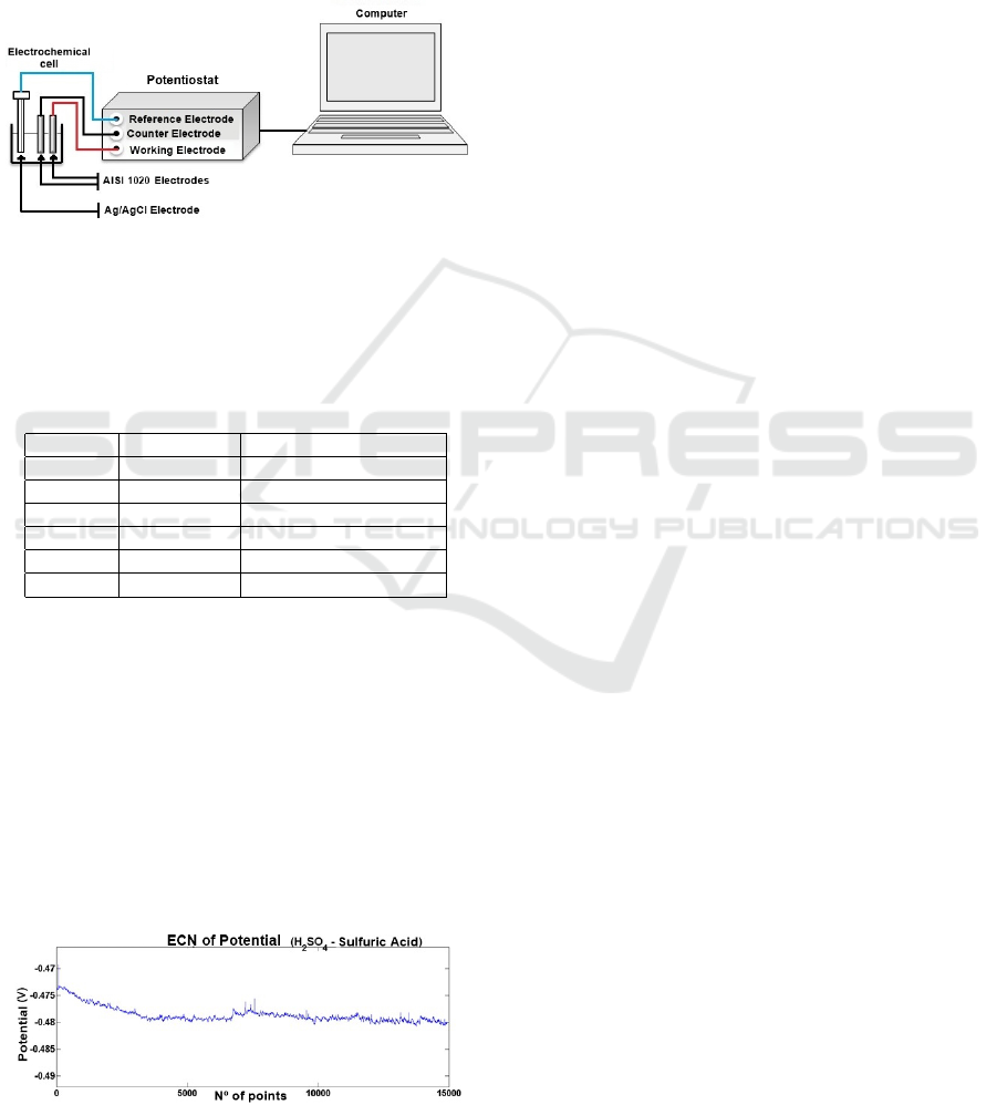
can be stored. Figure 1 shows a diagram with the in-
struments used for data collection.
Figure 1: Experimental apparatus configuration.
Table 1 shows the substances used in this work
and their applications. We have chosen substances
which are common in industrial environments.
Table 1: Used reagents and their concentrations (values in
mol/L) in aqueous solutions.
Substance Concentration Application
KCl 0.2, 0.4 and 0.6
Fertilizer production
NaOH 0.1, 0.2 and 0.3 Boilers
KOH 0.1, 0.2 and 0.3
Petrochemical industry
NaCl 0.2, 0.6 and 1.0
Cooling water
FeCl
3
0.1, 0.2 and 0.3
Coagulant in water treatment
H
2
SO
4
0.2, 0.3 and 0.4
Fertilizer production
The acquisition of the signals was obtained using
a potentiostat AUTOLAB
R
PGSTAT 101 Metrohm
model. This instrument is equipped with three con-
nections: working electrode, counter electrode and re-
ference electrode. The reference electrode used was
Ag/AgCl. To analyze the ECN measurements, for
each reagent was performed three different concen-
trations, totalizing 18 measurements with 60 minutes
each. The sampling frequency used was 4Hz, such
that each measurement has 14400 points. Figure 2
shows an example of measured signal.
Figure 2: Potential ECN signal.
4 EXPERIMENTS AND
DISCUSSION
The experiments were divided into two phases. In the
first phase was defined the size of data segments, that
is, the number of points of each sample before ex-
tracting the features. In the second phase, the classifi-
cation algorithms are trained with the features extrac-
ted by wavelet and RQA to identify the type of cor-
rosive substance. In both phases, the accuracy metric
was used as quality measure. The value of the accu-
racy is calculated by the ratio of the number of sam-
ples correctly classified by the total number of sam-
ples, multiplied by 100%.
4.1 Size of Data Segments
The features used to identify the type of substance are
extracted of several data segments. Therefore, it is
important to define its size, because few points per
segment supply little information, but, if is used many
points per segment, it will be impossible to evaluate
properly the proposed method. Thus, we evaluated
non-overlapping data segments in the range of 144 to
2880 points, with increments of 144 points. For this
experiment was used a total of 14400 points equally
distributed in all six classes, where 70% of the points
were used to train and the others 30% to test.
The first step of wavelet analysis method is to
remove the mean of each time series and to define
the corresponding wavelet family (father and mother)
(Aballe et al., 1999). The features used in this expe-
riment were computed from signal of potential with
Wavelet Transform of Daubechies (db4) with decom-
position at 8 levels. The main property of the Daube-
chies function is that it is a wavelet highly localized
in time, wich is good for electrochemical noise stu-
dies, where short time duration events are the norm
(Bertocci et al., 1997). The features extracted of each
non-overlapping data packets of ECN signal of po-
tential were: energy, entropy, detail and smooth coef-
ficients, as described in Section 2.1, resulting in a fe-
ature vector with 27 elements. These features were
selected with SBS algorithm (Sequential Backward
Feature Selection), which is a search algorithm that
starts with a complete set of features and for each ite-
ration removes the feature with the least impact on the
accuracy. Thus, only the most significant features are
kept (Dutra, 1999). After computing the features, they
were normalized by the mean and standard deviation.
To classification, we used a MLP (Multi-Layer
Perceptron) with 20 neurons in the hidden layer, le-
arning rate equal to 0.001 and 1000 training epochs
using Levenberg-Marquardt algorithm (Marquardt,
Identification of Corrosive Substances through Electrochemical Noise using Wavelet and Recurrence Quantification Analysis
721
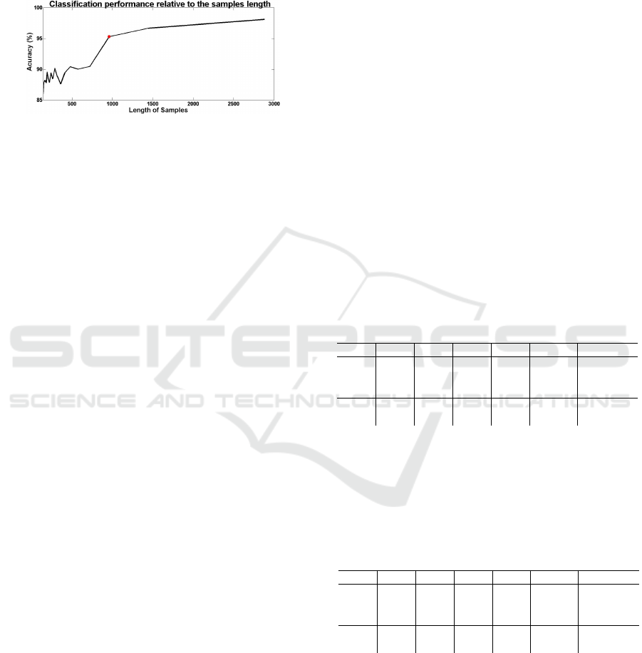
1963) for training. Figure 3 shows the accuracy va-
lues obtained for different numbers of points using
wavelet transform features. It is observed that the gre-
ater the number of points per segment, the better is the
accuracy.
Figure 3: Accuracy × sample length.
Ideally, a good choice is a large number of points
per segment (sample). However, the higher number of
points is, the smaller is the number of samples avai-
lable for training and testing. A compromise between
the two quantities is 960 points per segment, as indi-
cated in Figure 3. Therefore, we can have a reasona-
ble number of samples per class.
4.2 Corrosive Substances Identification
For these experiments, the features were extrac-
ted from non-overlapping data segments (samples)
of 960 points each, from electrochemical noise of
potential signals. Wavelet Transform of Daube-
chies (db4) with decomposition at 8 levels was
used to compute the energy and entropy, and de-
tail and smooth coefficients, resulting in a feature
vector with 27 elements. Similarly, RQA was
also used to extract features. The measures des-
cribed in Section 2.2 were extracted through the
RQA software 13.1 routines package, available at
http://homepages.luc.edu/∼cwebber/. Therefore, for
each sample was obtain a vector with 4 elements.
After this step, the samples were stratified into 3
folds of data, each one with 45 samples to each class.
Then, for each classifier were obtained 3 results from
3 tests, and each result was achieved using 2 folds
for training/validation and 1 fold for testing. For each
result was used a different fold for testing. The featu-
res were normalized by the mean and standard devi-
ation computed in the training folds. In this work we
used the following classifiers: MLP, PNN (Probabilis-
tic Neural Network) (Masters, 1995), kNN (k Nearest
Neighbor) (Duda et al., 2000), Decision Tree (Quin-
lan, 1988) and SVM (Support Vector Machines) (The-
odoridis and Koutroumbas, 2008) with linear (SVM-
L) and radial basis function (SVM-RBF) kernel.
The following configurations were tested for each
technique in order to maximize the accuracy on the
training set and, possibly, also on the test set. MLP
was trained using Levenberg-Marquardt algorithm,
learning rate of 0.001, 1000 epochs and evaluated dif-
ferent numbers of neurons in the hidden layer (1 to
50 neurons). Different values of standard deviation
were tested for PNN (0.1 to 1.0, with steps of 0.1).
For kNN, we employed Euclidean distance and we
varied the value of k (1 to 10). For SVM-L and SVM-
RBF, different values of cost c were evaluated (0 to
10, with steps of 0.5). Moreover, different values of
gamma (0.001 to 0.025, with steps of 0.005) were eva-
luated for SVM-RBF. For the decision tree was used
standard Matlab implementation, which does not have
parameters to tune. For each test, the parameters of
each technique were adjusted in order to maximize
the accuracy on the training folds, and these parame-
ters were used to classify the samples of the test fold.
Table 2 shows the values of the accuracy obtained
by each technique in each test fold when using wave-
let transform to feature extraction. The best result for
each fold is highlighted. As can be seen, MLP achie-
ved mean accuracy slightly better than those obtained
by the other classifiers, followed by SVM with linear
kernel.
Table 2: Classification results of each technique when using
wavelet to feature extraction (accuracy values are in per-
cent).
Test MLP PNN kNN Tree SVM-L SVM-RBF
1 95.56 71.97 90.48 84.76 87.66 87.66
2 97.14 75.00 94.29 89.52 94.28 92.38
3 95.87 68.94 86.67 81.90 91.42 90.47
Mean 96.19 71.97 90.48 85.40 91.12 90.17
Std. 0.008 0.030 0.030 0.038 0.033 0.023
Similarly, Table 3 shows the classification results
of each technique when using the features extracted
by RQA. As can be seen, decision tree achieved mean
accuracy slightly better than those obtained by the ot-
her classifiers.
Table 3: Classification results of each technique when using
RQA to feature extraction (accuracy values are in percent).
Test MLP PNN kNN Tree SVM-L SVM-RBF
1 91.11 94.44 94.44 97.78 83.33 86.67
2 92.22 88.89 90.00 92.22 88.88 91.11
3 78.89 86.67 88.89 87.78 81.11 78.89
Mean 87.41 90.00 91.11 92.59 84.44 85.56
Std. 0.074 0.040 0.029 0.050 0.040 0.061
The results in Tables 2 and 3 indicate that both ap-
proaches, wavelet transform and RQA, present a high
accuracy to perform detection of corrosive substan-
ces, but the best mean accuracy of wavelet transform
was slightly better than the results obtained by RQA.
Furthermore, we observed that MLP performance was
better when using features extracted by wavelet trans-
form, while decision tree was more effective when
ICPRAM 2017 - 6th International Conference on Pattern Recognition Applications and Methods
722

using features of RQA. This indicates some classi-
fiers are more appropriate to some type of features
than others. The authors did not find works with si-
milar objectives, but in the task of identifying types
of corrosion, as in (Jian et al., 2013) and (Hou et al.,
2016), that also use ECN signal, the accuracy is in the
range of 90% to 100%.
5 CONCLUSIONS
This paper presented an approach to identify some ty-
pes of reagents on metal surface through electroche-
mical noise signals using wavelet transform and re-
currence quantification analysis. Comparing the two
techniques, we noticed that both had a similar perfor-
mance, but wavelet transform was able to provide a
slightly higher average accuracy. For the classifiers
evaluated, we noted that MLP achieved an average
accuracy above 95% to perform the task. In relation
to the classification stage, the feature vector obtained
from the RQA is smaller, and requires less processing
capacity.
Therefore, the results of this study highlight the
importance of using wavelet transform and RQA for
electrochemical noise analysis. In future work, we in-
tend to analyze the combination of these methods, ot-
her algorithms and other features in order to improve
the results.
ACKNOWLEDGEMENTS
Lorraine Marques Alves would like to thank CAPES
for the scholarship granted.
REFERENCES
Aballe, A., Bethencourt, M., Botana, F., and Marcos, M.
(1999). Using wavelets transform in the analysis
of electrochemical noise data. Electrochimica Acta,
44(26):4805–4816.
Al-Mazeedi, H. and Cottis, R. (2004). A practical evalu-
ation of electrochemical noise parameters as indica-
tors of corrosion type. Electrochimica Acta, 49(17–
18):2787–2793.
Allegri, T. (2012). Handling and Management of Hazar-
dous Materials and Waste. Springer Science & Busi-
ness Media.
Bergelson, V. (2000). The multifarious poincaré recurrence
theorem. Descriptive set theory and dynamical sys-
tems, 1:31–57.
Bertocci, U., Gabrielli, C., Huet, F., and Keddan, M. (1997).
Noise resistance applied to corrosion measurements.
Electrochemical Society Journal, 144:31–37.
Cottis, R. A., Homborg, A., and Mol, J. (2015). The rela-
tionship between spectral and wavelet techniques for
noise analysis. Electrochimica Acta, pages 277–287.
Duda, R., Hart, D. G., and Stork, P. (2000). Pattern Recog-
nition. Wiley Interscience, New York, 1nd edition.
Dutra, L. (1999). Feature extraction and selection for ers-
1/2 insar classification. International Journal of Re-
mote Sensing, pages 993–1016.
Fofano, S. and Jambo, H. (2007). Corrosion: fundamentals,
monitoration and control. Ciencia Moderna, Brazil,
1nd edition.
Garcia-Ochoa, E. and Corvo, F. (2015). Using recurrence
plot to study the dynamics of reinforcement steel cor-
rosion. Protection of Metals and Physical Chemistry
of Surfaces, 51(4):716–724.
Hou, Y., Aldrich, C., Lepkova, K., Suarez, L., and Kinsella,
B. (2016). Monitoring of carbon steel corrosion by use
of electrochemical noise and recurrence quantification
analysis. Corrosion Science, pages 63–72.
Javaherdashti, R., Nwaoha, C., and Tan, H. (2013). Cor-
rosion and Materials in the Oil and Gas Industries.
CRC Press.
Jian, L., Weikang, K., Jiangbo, S., Ke, W., Weikui, W.,
Z.Weipu, and Zhoumo, Z. (2013). Determination of
corrosion types from electrochemical noise by artifi-
cial neural networks. international Journal of Elec-
trochemical Science, 8:2365–2377.
Koch, G., Varney, J., Thompson, N., Moghissi, O., Gould,
M., and Payer, J. (2016). International measures of
prevention, application and economics of corrosion
technologies study (impact). Technical report.
Marquardt, D. W. (1963). An algorithm for least-squares
estimation of nonlinear parameters. Journal of
the Society for Industrial and Applied Mathematics,
11(2):431–441.
Marwan, N., Romano, M., Thiel, M., and Kurths, J. (2007).
Recurrence plots for the analysis of complex systems.
Physics reports, 438:237–329.
Masters, T. (1995). Advanced algorithms for Neural Net-
works: A C++ Sourcebook. John Wiley and Sonsl,
New York, 1nd edition.
Montalban, L., Henttu, P., and Piche, R. (2007). Recur-
rence quantification analysis of electrochemical noise
data during pit development. International Journal of
Bifurcation and Chaos, 17:3725–3728.
Moshrefi, R., Mahjani, M., and Jafarian, M. (2014). Appli-
cation of wavelet entropy in analysis of electrochemi-
cal noise for corrosion type identification. Electroche-
mistry Communications, 48:49–51.
Quinlan, J. (1988). Decision trees and multivalued attribu-
tes. Oxford University Press, New York, 11nd edition.
Theodoridis, S. and Koutroumbas, K. (2008). Pattern Re-
cognition. Elsevier, San Diego, 4nd edition.
Identification of Corrosive Substances through Electrochemical Noise using Wavelet and Recurrence Quantification Analysis
723
