Triangular Curvature Approximation of Surfaces
Filtering the Spurious Mode
Paavo Nevalainen
1
, Ivan Jambor
2
, Jonne Pohjankukka
1
, Jukka Heikkonen
1
and Tapio Pahikkala
1
1
Dept. of Information Tech., Univ. of Turku, FI-20014 Turku, Finland
2
Dept. of Diagnostic Radiology, Univ. of Turku, FI-20014 Turku, Finland
{ptneva, ivjamb, jonne.pohjankukka, jukhei,tapio.pahikkala}@utu.fi
Keywords:
Curvature Spectrum, Parameterless Filtering, Irregular Triangulated Networks, Discrete Geometry.
Abstract:
Curvature spectrum is a useful feature in surface classification but is difficult to apply to cases with high noise
typical e.g. to natural resource point clouds. We propose two methods to estimate the mean and the Gaussian
curvature with filtering properties specific to triangulated surfaces. Methods completely filter a highest shape
mode away but leave single vertical pikes only partially dampened. Also an elaborate computation of nodal
dual areas used by the Laplace-Beltrami mean curvature can be avoided. All computation is based on trian-
gular setting, and a weighted summation procedure using projected tip angles sums up the vertex values. A
simplified principal curvature direction definition is given to avoid computation of the full second fundamental
form. Qualitative evaluation is based on numerical experiments over two synthetical examples and a prostata
tumor example. Results indicate the proposed methods are more robust to presence of noise than other four
reference formulations.
1 INTRODUCTION
Wide-scale point clouds have become accessible to
analysis everywhere. The point cloud surface regis-
tration typically has an approximate or accurate De-
launay triangular or tetrahedral mesh generation as a
preliminary step. The surface models are called irre-
gular triangularized networks (TIN) for historical re-
asons. The application domains can be roughly di-
vided to three categories by the target environment:
built environment, natural resource data and medical
3D imaging.
The ratio 0 ≤ σ
h
/r ≤ 0.3 of the perpendicular
noise component σ
h
and the nominal surface radius r
describe the difficulty of curvature registration. The
built environment data has usually high point den-
sity and small noise ratio compared to the natural re-
source data (Mitra and Nguyen, 2003). Built surfa-
ces are usually solid, curvature values change slowly
over distance, and it is desirable to be able to detect
the local curvature accurately. A typical mean curva-
ture method for such data is based on the Laplace-
Beltrami (L-B) operator (Meyer et al., 2003; Mes-
moudi et al., 2012).
Other two application domains have
the noise ratio much higher, approximately
σ
h
/r = 10
−2
...10
−1
(Schaer et al., 2007). Sur-
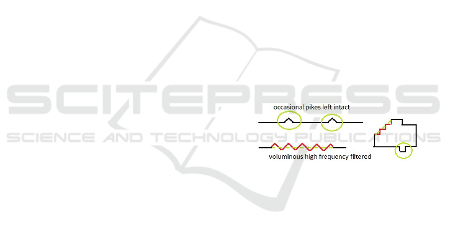
Figure 1: The voluminous highest noise component ari-
ses either from the scanning process (LiDAR point clouds,
left), or from the voxel granularity (right). Neither case
should require any parameters to filter. Occasional anoma-
lies (circles) should be transferred intact to pattern recogni-
tion phase.
faces, e.g. the terrain surface, are porous, covered
with vegetation or mathematically undefined. Natural
resource data is gatherer by aerial light detection
and ranging (LiDAR) or by spatial photogrammetry.
Natural resource data has shape recognition tasks
where the point samples per target ratio reaches
one (Nevalainen et al., 2016), i.e. one single elevated
hit is a possible target (e.g. a surface stone), see
Fig. 1. Detection of an individual target is naturally
uncertain in the presence of noise, but one can cluster
larger areas e.g. to stony or non-stony ones using
e.g. the curvature spectrum (Nevalainen et al., 2015).
On the other hand, there is a natural frequency limit
defined by the nominal mesh length. Excitation of
this frequency over a large area (see Fig. 1 left side) is
684
Nevalainen, P., Jambor, I., Pohjankukka, J., Heikkonen, J. and Pahikkala, T.
Triangular Curvature Approximation of Surfaces - Filtering the Spurious Mode.
DOI: 10.5220/0006249206840692
In Proceedings of the 6th International Conference on Pattern Recognition Applications and Methods (ICPRAM 2017), pages 684-692
ISBN: 978-989-758-222-6
Copyright
c
2017 by SCITEPRESS – Science and Technology Publications, Lda. All rights reserved

usually a numerical artifact which should be filtered
at some point of the processing.
Medical 3D applications, especially magnetic re-
sonance imaging (MRI), often have non-isotropic
voxels causing excitation at the frequency limit, see
right part of the Fig. 1. Numerical methods should be
resilient to effect of noise, low sampling and discreti-
zation patterns.
Surface registration is reminiscent of interpola-
tion, whereas noise reduction is filtering. Typically,
these two operations can be performed in any order, or
combined together. Spatial filtering requires several
parameters, and it is worthwhile to seek curvature re-
gistration methods, which would handle the highest
frequency as depicted in Fig. 1:
1. leaving single pikes to be handled by later pattern
recognition and filtering steps.
2. eliminating automatically large excitations of the
highest frequency.
Naturally, if such a behaviour is squarely against
the needs of a specific application, there is an abun-
dant supply of existing curvature registration met-
hods, which should be employed instead. Alternative
methods have several opposing properties for discrete
differential operators (Wardetzky et al., 2007) used as
building blocks for curvature analysis. If a new appli-
cation field arises, one has to be aware of the trade-
offs between different properties.
The Gaussian and mean curvature completely de-
fine the local curvature of any continuous surface. It
is the consensus of the current research that the local
Gaussian curvature is best estimated on TIN models
by so called angle deficit (see e.g. (Crane et al., 2013),
and the result is robust to noise. This reference met-
hod is named as vertex Gaussian in this paper.
This paper uses the classical differential geometric
definition of the average Gaussian curvature (Press-
ley, 2010): it is the ratio of the total orientation change
over a surface area, a TIN triangle in this case. It is
pointed out in Sec. 3.1 that this simple definition leads
to a triangular Gaussian curvature estimation on ver-
tices, which fills the requirements 1 and 2 mentioned
before.
The mean curvature is numerically more difficult
target than Gaussian curvature. One starting point for
computation has been neglected in the literature thus
far. It is possible to define the mean curvature by the
local rate of change of the surface area when the sur-
face is mapped towards the direction of its unit nor-
mal (Pressley, 2010). This definition is related to the
theory of minimal surfaces and it can be applied di-
rectly to the triangulated surface with defined vertex
normals. Also this novel mean curvature formulation
has the earlier mentioned properties 1 and 2, as rumi-
nated in Sec. 3.1.
The rest of the paper has the following struc-
ture: Section 2 introduces the triangular Gaussian and
mean curvatures, and a collection of competing defi-
nitions. Also the problem of finding the principal cur-
vature direction has been addressed there. Section 3
has a practical example (prostata tumor), and two
synthetical test cases to verify the properties 1 and 2
of the proposed method. Section 4 brings in the con-
clusions.
2 TRIANGULAR CURVATURE
The following notation will be used throughout the
presentation. The set of cloud points P ⊂ R
3
is gi-
ven. A triangle t = (a,b,c), a, b, c ∈ T ⊂ P
3
is de-
fined by three vertex points which can be referred in
cyclic fashion in counterclockwise order (with three
possible combinations considered identical). To shor-
ten the notation, the vertex membership a ∈ t and
the geometric insidence q ∈ t have the same nota-
tion, when the intended meaning is clear from the
context. A vertex p has a set of surrounding triang-
les T
p
= {t ∈ T |p ∈ t} ⊂ T . The edge neighborhood
N
p
= ∪
t∈T
p
t \{p} is a counterclockwise cyclically or-
dered set of points connected to p by a triangle edge.
The triangle t = {a, b,c} has a unique face normal
n
t
(oriented outwards) and an area A
t
:
N
t
= (b − a) × (c − a)
A
t
= kN
t
k/2 (1)
n
t
= N
0
t
, (2)
where N
t
is a temporary cross product term and vec-
tor power v
0
= v/kvk of a vector v denotes the vector
normalization.
Your Paper
You
November 15, 2016
Abstract
Your abstract.
φ
t
a
φ
t
p
a
b
t
p
n
p
n
t
References
1
Figure 2: Triangle concepts: tip angles φ
t p
are indexed by
vertices p of triangles t. Also the vertex normal n
p
and face
normal n
t
depicted.
The local curvature state of the surface is comple-
tely defined after finding out both mean curvature H
and the Gaussian curvature G. Sections 2.1- 2.7 pre-
sent the curvature quantities both in a triangle t and at
a vertex p.
Triangular Curvature Approximation of Surfaces - Filtering the Spurious Mode
685

2.1 Triangular Gaussian Curvature
The tangential orientation change ∆α over a length l
defines κ, the average of the curvature of a 2D curve
over the same length: κ = ∆α/l. Analogous to this,
the average of the Gaussian curvature of a smooth sur-
face S ⊂ R
3
can be defined (Pressley, 2010, p.166-
168) as the ratio G
S
= ω
S
/A
S
, where A
S
is the surface
area of S and ω
S
is the solid angle of which the sur-
face normal n(q),q ∈ S traces. This definition can be
applied to a triangle t = {a,b,c} with vertex normals
n
a
,n
b
,n
c
with the exception that the accurate surface
S is not known and the triangle area A
t
is a lower
bound approximation of the hypothetical smooth area
meas(S
q
). Ramifications of this fact will be addressed
in Sec. 3.1.
The solid angle ω
t
in Eq. 3 is the total trace of
normal n(q), q ∈ t and, assuming a barycentric inter-
polation scheme, it equals the solid angle of a vec-
tor tri-blade n
a
, n
b
, n
c
(van Oosterom and Strackee,
1983):
tan(ω
t
/2) =
n
a
·n
b
×n
c
1+n
a
·n
b
+n
b
·n
c
+n
c
·n
a
(3)
G
t
= ω
t
/A
t
. (4)
The numerator in Eq. 3 equals zero when at least two
vertex normals are parallel, which results in require-
ments 1 and 2 of Sec. 1 to be fulfilled as far as trian-
gular Gaussian G
t
of Eq. 4 is concerned. This will be
elaborated further in Sec. 3.1.
2.2 Triangular Mean Curvature
Considering a triangle t = (a,b,c) and the associa-
ted surface normal approximants n
a
,n
b
,n
c
at verti-
ces a,b,c, and a barycentric dependency of normals
n(q),q ∈ t in the triangle t, one can define a nor-
mal mapped parallel triangle t
u
= {q + u n(q)|q ∈ t}.
Using a definition of (an averaged) mean curvature
in (Pressley, 2010, p. 207), one gets:
H
t
=
1
2A
t
d
du
A
t
u
|
u=0
=
(n
b
−n
a
)×(c−a)+(b−a)×(n
c
−n
a
)
4A
t
· n
t
. (5)
Note that triangular mean curvature H
t
≡ 0 when all
the vertex unit normals are parallel i.e. n
a
= n
b
= n
c
.
This leads to requirements 1 and 2 of Sec. 1 to be
fulfilled.
2.3 Projective Tip Angles as Weights
The vector angle function acos() and the projected
vector angle function acos
n
() simplify the upcoming
presentation. The projection angle φ
0
12
is the angle φ
0
12
between vectors v
1
and v
2
when seen from direction
n. See the right part of the Fig. 3. A projection matrix
P(n) = I − n
0
n
0T
is used to define acos
n
(.):
acos(v
1
,v
2
) = cos
−1
(v
0
1
· v
0
2
) (6)
v
0
i
= P(n)v
i
, i = 1,2
acos
n
(v
1
,v
2
) = acos(v
0
1
,v
0
2
). (7)
Note that acos(v
1
,v
2
) ≡ acos
v
1
×v
2
(v
1
,v
2
).
Your Paper
You
November 21, 2016
Abstract
Your abstract.
a
b
c
p
t
1
t
2
φ
t
2
c
φ
t
1
a
v
1
v
2
n
φ
12
φ
0
12
v
0
1
v
0
2
References
1
Figure 3: Left: the angle φ
12
between two vectors v
1
,v
2
and
the projected angle φ
0
12
between projected vectors v
0
1
,v
0
2
.
Right: Definition of the edge angles φ
0
t
0
q
and φ
t
0
q
0
of an edge
(p,q).
The projective tip angles φ
0
t p
are used systemati-
cally to average all triangular quantities X
t
, t ∈ T to
corresponding vertex quantities X
p
, p ∈ P :
φ
0
t
1
a
= acos
n
p
(p − a, b − a) ( See Fig. 3) (8)
φ
0
p
=
∑
t∈T
p
φ
0
t p
(9)
X
p
=
∑
t∈T
p
φ
0
t p
X
t
/φ
0
p
. (10)
This weighting procedure of a quantity X will be de-
noted as: X
t
→ X
p
in the rest of the text.
Good numerical properties of tip angle weighting
pointed us to amortize the computational costs by ap-
plying it to produce the following vertex properties:
normals n
p
, triangular mean curvature H
p
, triangu-
lar Gaussian G
p
and principal curvature direction v
p
.
Another benefit was the unified handling of the boun-
dary points, since the angle sums φ
0
p
≤ φ
p
≤ 2π give
an excellent weighting at the boundary. This is impor-
tant because e.g. the natural resource data is prune to
have missing values and holes in the point cloud, and
the boundary points are thus common. When a point
p is not in the border, the sum of projected angles
equals: φ
0
p
≡ 2π. There are other weighting schemes
in the literature, these are being discussed in Secti-
ons 2.5 and 2.6.
2.4 Vertex Gaussian
Since the projected tip angles have been introduced,
it is possible to define an alternative vertex Gaussian
using the spherical excess (Crane et al., 2013) formu-
lation. The vertex Gaussian of Eq. 12 serves as a re-
ICPRAM 2017 - 6th International Conference on Pattern Recognition Applications and Methods
686

ference method:
φ
p
=
∑
t∈T
p
φ
t p
(11)
G
p
= (φ
0
p
− φ
p
)/(A
p
/3). (12)
2.5 Vertex Normals
Vertex normals n
p
are weighted from triangle normals
n
t
using the generic scheme of projected tip weighting
defined in Eq. 10: n
t
→ n
p
. There are several other
possible definitions. Vertex normals can be conside-
red pointing towards the new altered vertices after the
local surface is varied, or they somehow represent a
continuous but unknown reference positions. The al-
ternatives satisfying DDG convergence requirements
listed in (Crane et al., 2013) are reproduced here for
discussion. The vertex normal can be:
1. The vector area: n
p
=
∑
t∈T
p
A
t
n
t
0
2. The area (or volume) gradient n
p
= (dA
p
/d p)
0
,
when one vertex p is varied in R
3
.
3. The normal of a sphere which inscribes vertex p
and its edge-neighborhood points N
p
. See (Max,
1999; Crane et al., 2013).
Such a sphere fitting required by the alternative 3 is
impossible with usual point clouds, but just applying
the definition from a case of a perfect sphere fit to any
general triangle neighborhood, the resulting normal
vector n
p
behaves smoothly:
n
p
=
∑
t=(a,p,b)∈T
p
n
t
kb − pkka − pk
0
.
According to (Jin et al., 2005), versions 1 and 2 are
simple but prune to noise, projected tip angle weig-
hting (our choice) is reliable and simple, and version
3 is rather good but also somewhat expensive.
2.6 Other Mean Curvature Definitions
This short survey omits all methods based on a local
fit of a smooth interpolant, see e.g. (Yang and Qian,
2007). These methods show resilience to noise, but
tend to have an uncontrollable loss of high frequen-
cies and are usually computationally more expensive
than the methods presented in the following.
The mean curvature through the discrete Laplace-
Beltrami (also known as the cotan-Laplace) operator
has been documented in (Mesmoudi et al., 2012). It
is one of the best methods according to (Mesmoudi
et al., 2012). The mean curvature H
p
at a vertex p
becomes:
H
p
=
1
4A
0
p
k
∑
b∈N
p
(
1
tanφ
t
1
a
+
1
tanφ
t
2
c
)(b − p)k, (13)
where triangles t
1
,t
2
∈ T
p
have a common edge (p, b)
with opposite vertex angles φ
t
1
a
,φ
t
2
b
. See Fig. 3. The
vertex specific area A
0
p
≈ A
P
/3 is the area of so called
mixed Voronoi cell. Using A
0
p
instead of A
p
/3 reduces
the area contribution of possible obstuse angles φ
t p
in
a way, which is detailed in (Mesmoudi et al., 2012).
The exact value of A
0
p
depends on the geometry of
the triangle set T
p
but is always rather close to the
above given expected average. The variance in A
0
p
adds numerical stability of the estimates of the vertex
mean curvature H
p
but is rather costly to calculate.
Your Paper
You
November 15, 2016
Abstract
Your abstract.
a
b
t
1
t
2
q
p
n
t
1
n
t
2
β
t
1
t
2
References
1
Figure 4: The edge angle β
t
1
t
2
is positive when the edge
folds downwards (or inwards in case of tumors).
The concentrated Gaussian curvature by (Mes-
moudi et al., 2012) equals Eq. 12. The concentrated
mean curvature by (Mesmoudi et al., 2012) is re-cast
to the notation in this paper as:
sgn(t
1
,t
2
) = −sgn((b − p) · n
t
1
) (14)
β
t
1
t
2
= acos(n
t
1
,n
t
2
)sgn(t
1
,t
2
) (15)
ω
p
= 2π −
∑
t
1
∈T
p
β
t
1
t
2
(16)
H
p
=
1
4A
0
p
(2π − ω
p
), (17)
where the edge angles β
t
1
t
2
are depicted in Fig. 4,
the angle sum ω
p
is the inwards opening solid angle
at vertex p, and the summation is done over edges
(p,q), q ∈ N
p
.
The sign of the edge angle β
t
1
t
2
is determined by a
vector blade handedness sign (a determinant sign) of
an edge (p,q) = t
1
∩t
2
between triangles t
1
= (a, p,q)
and t
2
= (q, p,b), see Eq. 14. Note that the edge sign
is positive for pikes (the situation depicted in Fig. 4)
and symmetric: sgn(t
1
,t
2
) = sgn(t
2
,t
1
). The normals
n
t
are a result of earlier stages of the computational
process.
Also the solid angle ω
p
in Eq. 17 is already avai-
lable from the preceding solid angle filtering (SAF),
which can be done to reduce the noise level of the
point cloud or for filtering out the foliage signal (Ne-
valainen et al., 2016), or before any shape classifica-
tion via curvature spectrum. Availability of spatial an-
gles ω
p
makes this method computationally the chea-
pest one.
Triangular Curvature Approximation of Surfaces - Filtering the Spurious Mode
687

In some applications like tumor detection in elec-
tron magnetic resonance (EMR) imaging, the orienta-
tion of the surface normal n
p
is completely free (but
outwards from the tumor). That is why the edge sig-
num refers only to two adjoined triangles t
1
and t
2
which are both oriented outwards. The signum in
Eq. 15 requires one vector operation (saxpy, see (Go-
lub and Van Loan, 1996)) of R
3
vectors.
Barycentric interpolation (Theisel et al., 2004) is
based on normalized linear change of the normal n
over the triangle t from where a generic expression
for Gaussian and mean curvature can be deduced. For
our purposes only the mean curvature H
t p
of triangle
t = (a,b,c) at a vertex point p ∈ {a, b,c} needs to
be considered. The Eq. 18 is adapted to our notation
from (Theisel et al., 2004; Nevalainen et al., 2015):
h = n
a
× (c − b) + n
b
× (a − c) + n
c
× (b − a)
H
t p
= (n
p
· h)/(2n
p
· N
t
) (18)
H
t p
→ H
p
, (19)
where h is a temporary vector multiplicant.
There is also a triangular approximation of the se-
cond fundamental form (Crane et al., 2013; Rusinkie-
wicz, 2004), which is used in (Rusinkiewicz, 2004)
to derive the principal curvatures, mean and Gaussian
curvature principal and directions directly. This met-
hod requires iteration of a least squares problem, and
it seems to be computationally more expensive than
the methods covered here.
There are other possible interpolation schemes
over a triangle, e.g. using radial basis or by applying
the well-known Rodriguez rotation formula (Dorst
et al., 2007) twice (first over one edge, then between
edge and a vertex of interest). Preliminary tests indi-
cate that these options seem to lead to more complex
formulas yet the numerical results stay very close to
the schemes included to this study. This holds to both
the triangular and the vertex values.
2.7 Principal Curvature Orientation
The curvature eigenvalues κ
t1
and κ
t2
of a triangle t
are the curvature extremals when tracing a continuous
surface S through point p by a perpendicular plane:
κ
tl
= H
t
±
q
H
2
t
− G
t
,l = 1,2 (20)
Object and shape recognition may use any subset of
the four curvature characteristics G,H,κ
1
,κ
2
.
The barycentric surface normal map t → t
u
was
used to derive Eq. 5. By applying it again, but this
time to find a trajectory with most drastic curvature
effect per traversed arc length on a triangle t, one gets
the principal curvature direction v
t
of a triangle t. This
is a direction with the largest curvature (eigenvector
of κ
1
). The second eigenvector is not of interest, since
it will be dictated by the first eigenvector. Another
Figure 5: Averaging principal curvature direction v
t
from
triangles (above) to vertices v
p
(below).
way to express v
t
is based on constraining the second
fundamental form to be diagonal and solving the prin-
cipal direction from this constraint at Eq. 21. This is
different from (Rusinkiewicz, 2004), where whole the
second fundamental form is solved by least squares
fitting a set of linear constraints. Below are the equa-
tions leading to the eigenvalue problem:
0
m
a
= P(b − c)(a − c) (before scaling)
0
m
b
= P(a − c)(b − c) (before scaling)
m
a
=
0
m
a
0
m
a
·(a−c)
m
b
=
0
m
b
0
m
b
·(b−c)
D
t
= (n
a
− n
c
)m
T
a
+ (n
b
− n
c
)m
T
b
P(n
t
)D
t
v
t
= λv
t
, (21)
where
0
m
a
,
0
m
b
,m
0
a
m
b
are constituents of a constant
matrix D
t
= dn
t
/dq, the rate of change of the normal
at triangle t. Note that eigenvalue λ is not proportional
to principal curvature, since the barymetric mapping
does not preserve the unity of the normals.
The weighted summation scheme v
t
→ v
p
of
Eq. 10 is not directly applicable, since the principal
directions ±v
t
are defined by the orientation only, wit-
hout a coherent sign. The summation must take this
into account. The following heuristics relies on the
monotonic nature of the vector summation of the non-
unit cumulative vector ˆv
p
:
ˆv
p
(S) = P(n
p
)
∑
t∈T
p
φ
0
t p
sgn
t p
v
t
S
∗
= argmax
S
k ˆv
p
(S)k
v
p
= ( ˆv
p
(S
∗
))
0
, (22)
where S is the set of signums S = {sgn
t p
}
t∈ T
p
, which
can be found performing O(|T
p
|) scalar products
ICPRAM 2017 - 6th International Conference on Pattern Recognition Applications and Methods
688

ˆv
p current
· v
t
by a single enumeration and reversing a
subset of signums if necessary.
The weighting scheme in Eq. 22 relies on the pro-
jected tip angle weights φ
0
t p
, which have multiple ap-
plications and thus can be amortized from computa-
tional cost. The weighting scheme in (Rusinkiewicz,
2004) uses triangular contributions of the vertex spe-
cific area A
0
p
. This weighting scheme has not been
tested by us. Overall, avoiding the least squares fit
and area weighting makes our method less expensive
computationally.
3 NUMERICAL EXPERIMENTS
Two synthetical models and a visual inspection of
a practical problem have been covered, see Secti-
ons 3.1- 3.3. The following mean curvature methods
have been compared:
1. triangular average mean curvature (our method)
2. L-B (Meyer et al., 2003)
3. concentrated mean curvature (Mesmoudi et al.,
2012)
4. barycentric interpolation of the normal (Theisel
et al., 2004)
Two Gaussian curvatures have been compared, trian-
gular average Gaussian (our method, Eq. 4), and ver-
tex Gaussian (Crane et al., 2013). Since there are 3
vertex normal definitions, 2 weighted summation po-
licies, 4 mean curvature and 2 Gaussian curvature de-
finitions, results of only the most interesting combi-
nations have been provided.
3.1 A Local Pike
This model demonstrates the different character of
each methods with respect to noise in the surface nor-
mal direction. Especially the two noise modes presen-
ted in Fig. 1 are modelled. The case 1 in Fig. 6 is an
apex of a larger regular formation. The case 2 is a sin-
gle pike which can be either noise or a useful feature.
The case 3 demonstrates a large noise field at the hig-
hest possible frequency dictated by point cloud den-
sity. The geometrical mean
p
|G| = κ
G
derived from
the Gaussian curvature G is used for the comparisons,
since it has the same physical dimension (inverse of
radius) as the mean curvature.
The abscissa value h is the height of point p.
When h → 0, it is the planar special case with nominal
radius r → ∞ and κ r → 1.
The barycentric method exaggerates curvature at
large h values, which are likely to be noise. The bary-
centric mean curvature and the triangular curvatures
10
a local pike, cases 1,2,3
-1
0
5
2
1
0
0
-2
-2 -1 0 1 2
h
-0.5
0
0.5
1
1.5
2
r
case 1
triang. H
L-B H
concen. H
baryc. H
vertex G
triang. G
-2 -1 0 1 2
h
-0.5
0
0.5
1
1.5
2
r
case 2
-2 -1 0 1 2
h
-0.5
0
0.5
1
1.5
2
r
case 3
Figure 6: Four mean curvature methods and two Gaussian
curvature methods compared in various settings with one
point protruding out. The square root of the Gaussian cur-
vature is used for comparison. The analysis point at height
h has been circled.
(our methods, both G and H) tend to dampen a sin-
gular pike (case 2). The barycentric method is losing
its dampening tendency at high values of h, which are
more likely to be noise.
The output value of the vertex mean and Gaussian
curvatures (and barycentric mean curvature) is scaled
downwards (dampened) by a ratio w, value of which
depends on the case. The cases 1, 2,3 have dampe-
ning ratios w = 1, 1/3, 0. A singular pike (case 2) has
dampening factor 1/3 which is still adequate to con-
tribute in the curvature spectrum or to be detected by
later pattern recognition phase.
The egg cell pattern of case 3 gets completely
dampened by triangular curvatures G and H, and by
the barycentric method. The vertex normals defined
by Eqs. 2 and 10 become parallel, which then cau-
ses the triangular curvatures of the involved triangles
t to be zero, see Eqs. 5 and 4. This can be a use-
ful property in some applications, e.g. in stone de-
tection (Nevalainen et al., 2016), or in reducing the
granularity effect produced by voxels.
The concentrated curvature, vertex Gaussian, and
Laplace-Beltrami are closely related in all cases. The
behaviour of all six methods is rather similar to each
other in the hyperbolical case (a saddle point) and this
case has not been included in this presentation.
3.2 A Torus
A torus of radii r = 1, R = 2.5 has been used. This is
a classical test case, since the curvature aspects of the
ideal shape are analytical, yet both elliptic and hyper-
Triangular Curvature Approximation of Surfaces - Filtering the Spurious Mode
689
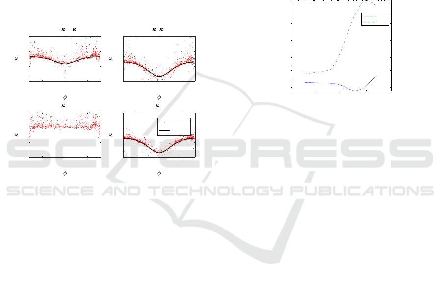
bolic local surface metrics occurs.
Two torii, a dense one with |P | = 820 and a sparse
one with |P | = 220 were used. Fig. 7 shows the sparse
torus with uniform local height distribution. A uni-
form distribution is used also on the tangential mani-
fold metrics. The height noise concerns point loca-
tions and the tangential noise concerns triangulation
irregularity. The height noise std. was varied between
0 ≤ σ
h
≤ 0.3r. The upper end of the noise is typi-
cal to many LiDAR applications. The height noise
distributions from real LiDAR data are not uniform
nor Gaussian. The main curvature spectrum seems to
depend mainly on the std of the uniform or natural
height distribution, not from the choice between the
two.
-2 0 2
-1
0
1
2
0.5*(
1
+
2
)
-2 0 2
-1
0
1
2
1 2
-2 0 2
-1
0
1
2
1
-2 0 2
-1
0
1
2
2
triang.
ideal
Figure 7: The triangular mean curvature and triangular
Gaussian curvature and two curvature eigenvalues on a to-
rus as a function of the angle φ associated with the smaller
radius. The height noise is at the maximum σ
h
/r = 0.3.
3.3 A Prostate Tumor
The main difficulty with MRI point clouds arises from
the anisotropy of the point cloud. The voxels are
elongated 2.75 × 0.48 × 0.48 mm
3
and this demands
a lot from the curvature analysis methods. Informa-
tion about the curvature spectrum of the tumor has
been applied to e.g. breast cancer classification (Lee
et al., 2015). It is possible that the curvature spectrum
will be an important feature alongside spatial texture
patterns, 3D Fourier transform, overall size and loca-
tion of the tumor for clustering algorithms. The Gaus-
sian curvature and principal curvature direction can
help in e.g. descriptor based vectorization (Vranic
and Saupe, 2001). Fig. 10 depicts a prostate lesion,
which shows a typical developable shape: the lesion
could be spread back to planar (its Gaussian curvature
is approximately zero).
3.4 Results
Our method, when referred, means triangular mean
and Gaussian (Eqs. 5, 4, 10) and the principal curva-
tures derived from them. Tests reach the high noise
amplitude range σ
h
/r = 0.3 typical to the natural re-
source data, see Fig. 7. Effects of noise filtering of L-
B and our method have been depicted in Fig. 8. L-B
is bound by its fidelity to local geometry. Difference
at smooth surface (the left part of the abscissa) is due
to the irregularity of the triangles, which brings some
advantage to an averaging method like ours.
10
−4
10
−3
10
−2
10
−1
10
0
0.3
0.4
0.6
0.8
1
2
4
σ
h
/r
RMSE(H)
Effect of height noise to mean curvature error
triang.
LB
Figure 8: The root mean square error of the mean curva-
ture H estimation error under different perpendicular noise
levels σ
h
(std.) on a torus with radii r and R.
Fig. 9 has curvature spectrae based on L-B and
our method. Other methods were inferior at the noisy
end and had to be excluded. The presence of noise
spreads the detected spectrum from the ideal smooth
case. L-B manages the task only if the triangulariza-
tion is rather regular and the height noise almost zero.
Our method captures two-thirds of the mean curva-
ture distribution, yet suffers from the spectrum spread
caused by the noise, which is inevitable. Both Gaus-
sian approximations perform as well enabling e.g. the
curvature spectrum classification to be possible under
wide range of noise levels. Other two methods (con-
centrated and barycentric) perform worse than L-B.
Fig. 10 depicts the prostate lesion with the Gaus-
sian curvature close to zero everywhere meaning its
surface is mostly developable (a so called ruler sur-
face). This is an artifact caused by a combination of
the elongated voxels and the method used for trian-
gularization. The surface has high energy noise com-
ponent caused by the voxel granularity. Our methods
dampen this highest geometric noise component au-
tomatically. Also concentrated and barycentric mean
curvatures performs surprisingly well. L-B suffers
from its fidelity to the highest shape frequency com-
ponent.
The computational cost of the barycentric method
is too high when compared to its performance, see
ICPRAM 2017 - 6th International Conference on Pattern Recognition Applications and Methods
690
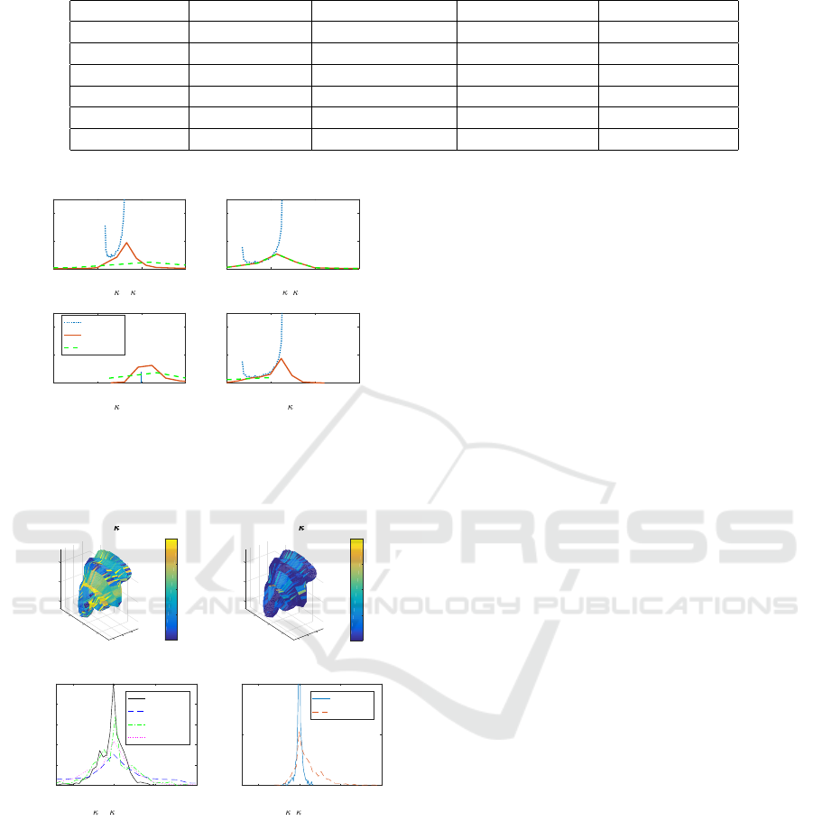
Table 1: Evaluation of the mean curvature methods. Proposed methods in boldface.
Method Vector opers/t Spectrum quality Singular noise w Massive noise w
vertex G 15 good 1 1
triangular G 15 good 1/3 0
triangular H 15 good 1/3 0
LB 18 average 1 1
concentrated 2 poor 1 1
barycentric 32 poor 1/3 0
-1 0 1 2
0.5*(
1
+
2
)
0
2
4
f
-1 0 1 2
1 2
0
2
4
f
-1 0 1 2
1
0
2
4
f
-1 0 1 2
2
0
2
4
f
ideal
triangular
L-B
Figure 9: The ideal curvature spectra of a torus with r = 1,
and Laplace-Beltrami and triangular approximations. The
effect of height noise σ
h
/r = 0.1 spreads out the approxi-
mated spectrae.
160
170
170
180
x,y,z (mm)
160
triangul.
1
40
150
30
-0.1
0
0.1
0.2
0.3
mm
-1
160
170
170
180
x,y,z (mm)
160
triangul.
2
40
150
30
-0.1
0
0.1
0.2
0.3
mm
-1
-0.5 0 0.5 1
(
1
+
2
)/2 (mm
-1
)
0
1
2
3
4
5
f
mean curvature H
triangular
L-B
concentr
barycentr
-0.5 0 0.5 1
1 2
(mm)
-2
0
5
10
f
Gaussian curvature G
triangular
vertex
Figure 10: Upper row: the principal curvature components.
Lower row: Distributions of the mean and Gaussian curva-
tures by different methods.
Table 1. L-B has the best accuracy when the perpen-
dicular noise is small and the triangulation is rather
regular, but fails when the perpendicular noise is high.
The spectrum quality is given a qualitative judgement.
See the definition of the dampening ratio w at Sec. 3.1.
4 CONCLUSIONS
The proposed method (triangular mean and Gaussian
curvature) has about the same computational demand
as the reference method (LB mean and vertex Gaus-
sian curvature) in case where the vertex specific area
A
0
p
of the mixed Voronoi cell is computed exactly as
recommended in (Mesmoudi et al., 2012). Based on
the good performance under height noise, it seems
that the triangular method should be used in such na-
tural resource data applications, where the curvature
spectrum is required, and the spectral range should
reach near the highest shape frequency, but excluding
the large excitations of the mentioned frequency.
The above definition may seem contrived, but e.g.
a typical rasterization process is lossy and tuning the
filtering process requires a lot of parameters, which
concern the highest shape frequency naturally contai-
ned with the methods proposed here. Further valida-
tion is necessary with e.g. track analysis of forestry
harvesters (Pierzchala et al., 2016).
Principal orientation computation presented in
Sec. 2.7 is closely related to other two methods pre-
sented, e.g. it uses the same projected tip angle weig-
hts. One has to inspect in the future how useful the
principal orientations are in micro-topographic analy-
sis. It may be that a multi-scale approach for produ-
cing several TIN models with coherent curvature and
principal orientation information is needed.
There is a huge bulk of raster analysis methods
and a lot of experience in applying these methods for
e.g. height raster data analysis. Emerging triangular
analysis tools based on DDG will not outdate these
methods, but in some cases there seems to be potential
to improve the curvature spectrum range closer to the
theoretical limit dictated by the point cloud sample
density and the known sample accuracy.
ACKNOWLEDGEMENTS
This work was supported by the funding from the
Academy of Finland (Grant 295336). Kevin R. Vixie
Triangular Curvature Approximation of Surfaces - Filtering the Spurious Mode
691

and Otis Chodosh brought up the intuitive view to
mean curvature on Math Overflow site on 2012.
REFERENCES
Crane, K., de Goes, F., Desbrun, M., and Schr
¨
oder, P.
(2013). Digital geometry processing with discrete ex-
terior calculus. In ACM SIGGRAPH 2013 Courses,
SIGGRAPH ’13, pages 7:1–7:126, New York, NY,
USA. ACM.
Dorst, L., Fontijne, D., and Mann, S. (2007). Geometric
Algebra for Computer Science: An Object-Oriented
Approach to Geometry. Morgan Kaufmann Publishers
Inc., San Francisco, CA, USA, 1st edition.
Golub, G. H. and Van Loan, C. F. (1996). Matrix Com-
putations (3rd Ed.). Johns Hopkins University Press,
Baltimore, MD, USA.
Jin, S., Lewis, R., and West, D. (2005). A comparison of
algorithms for vertex normal computation. The Visual
Computer, 21:71–82.
Lee, J., Nishikawa, R. M., Reiser, I., Boone, J. M., and
Lindfors, K. K. (2015). Local curvature analysis for
classifying breast tumors: Preliminary analysis in de-
dicated breast ct. Medical Physics, 42(9).
Max, N. (1999). Weights for computing vertex normals
from facet normals. Journal of Graphics Tools, 4(2).
Mesmoudi, M. M., De Floriani, L., and Magillo, P. (2012).
Discrete curvature estimation methods for triangula-
ted surfaces. In Applications of Discrete Geometry
and Mathematical Morphology, pages 28–42. Sprin-
ger.
Meyer, M., Desbrun, M., Schr
¨
oder, P., and Barr, A. H.
(2003). Visualization and Mathematics III, chapter
Discrete Differential-Geometry Operators for Trian-
gulated 2-Manifolds, pages 35–57. Springer Berlin
Heidelberg, Berlin, Heidelberg.
Mitra, N. J. and Nguyen, A. (2003). Estimating surface
normals in noisy point cloud data. In Proceedings of
the Nineteenth Annual Symposium on Computational
Geometry, SCG03, pages 322–328, New York, NY,
USA. ACM.
Nevalainen, P., Middleton, M., Kaate, I., Pahikkala, T., Su-
tinen, R., and Heikkonen, J. (2015). Detecting stony
areas based on ground surface curvature distribution.
In 2015 International Conference on Image Proces-
sing Theory, Tools and Applications, IPTA 2015, Orle-
ans, France, November 10-13, 2015, pages 581–587.
Nevalainen, P., Middleton, M., Sutinen, R., Heikkonen, J.,
and Pahikkala, T. (2016). Detecting terrain stoniness
from airborne laser scanning data . Remote Sensing,
8(9):720.
Pierzchala, M., Talbot, B., and Astrup, R. (2016). Mea-
suring wheel ruts with close-range photogrammetry.
Forestry, 89(4):383–391.
Pressley, A. (2010). Elementary Differential Geometry.
Springer Undergraduate Mathematics Series. Springer
London.
Rusinkiewicz, S. (2004). Estimating curvatures and their
derivatives on triangle meshes. In Symposium on 3D
Data Processing, Visualization, and Transmission.
Schaer, P., Skaloud, J., Landtwing, S., and Legat, K. (2007).
Accuracy Estimation for Laser Point Cloud Including
Scanning Geometry. In Mobile Mapping Symposium
2007, Padova.
Theisel, H., R
¨
ossl, C., Zayer, R., and Seidel, H. P. (2004).
Normal based estimation of the curvature tensor for
triangular meshes. In In PG04: Proceedings of the
Computer Graphics and Applications, 12th Pacific
Conference on (PG2004), pages 288–297. IEEE Com-
puter Society.
van Oosterom, A. and Strackee, J. (1983). A solid angle of a
plane triangle. IEEE Trans. Biomed. Eng., 30(2):125–
126.
Vranic, D. V. and Saupe, D. (2001). 3d shape descriptor
based on 3d fourier transform. In Fazekas, K., edi-
tor, 3D Shape Descriptor Based on 3D Fourier Trans-
form In Proceedings of the EURASIP Conference on
Digital Signal Processing for Multimedia Communi-
cations and Services (ECMCS 2001), pages 271–274.
Wardetzky, M., Mathur, S., Kaelberer, F., and Grinspun, E.
(2007). Discrete laplace operators: No free lunch. In
Belyaev, A. and Garland, M., editors, Geometry Pro-
cessing. The Eurographics Association.
Yang, P. and Qian, X. (2007). Direct computing of surface
curvatures for point-set surfaces. In SPBG’07, pages
29–36.
ICPRAM 2017 - 6th International Conference on Pattern Recognition Applications and Methods
692
