Deep Learning Approach for Classification of Mild Cognitive
Impairment Subtypes
Upul Senanayake
1
, Arcot Sowmya
1
, Laughlin Dawes
2
, Nicole A. Kochan
3
, Wei Wen
3
and Perminder Sachdev
3
1
School of Computer Science and Engineering, UNSW, Sydney, Australia
2
Prince of Wales Hospital, Randwick, Sydney, Australia
3
Centre for Healthy Brain Ageing, UNSW, Sydney, Australia
Keywords:
Alzheimer’s Disease, Mild Cognitive Impairment, Deep Learning, Neuropsychological Features.
Abstract:
Timely intervention in individuals at risk of dementia is often emphasized, and Mild Cognitive Impairment
(MCI) is considered to be an effective precursor to Alzheimers disease (AD), which can be used as an inter-
vention criterion. This paper attempts to use deep learning techniques to recognise MCI in the elderly. Deep
learning has recently come to attention with its superior expressive power and performance over conventional
machine learning algorithms. The current study uses variations of auto-encoders trained on neuropsycholog-
ical test scores to discriminate between cognitively normal individuals and those with MCI in a cohort of
community dwelling individuals aged 70-90 years. The performance of the auto-encoder classifier is further
optimized by creating an ensemble of such classifiers, thereby improving the generalizability as well. In ad-
dition to comparable results to those of conventional machine learning algorithms, the auto-encoder based
classifiers also eliminate the need for separate feature extraction and selection while also allowing seamless
integration of features from multiple modalities.
1 INTRODUCTION
A decline in cognitive functions such as memory,
processing speed and executive processes is associ-
ated with aging by Hedden and Gabrieli (Hedden
and Gabrieli, 2004). Every human will eventually
go through this process in varying degrees from dif-
ferent starting points and different rates of progres-
sion (Chua et al., 2009; Cui et al., 2012a; Gauthier
et al., 2006). Since cognitive decline in late life is
commonly associated with brain pathology, it has be-
come an ongoing research challenge to discriminate
between cognitive decline due to pathological pro-
cesses and normal aging. Among the numerous neu-
rodegenerative diseases, Alzheimer’s disease (AD) is
at the forefront, as the progressive cognitive impair-
ment caused by it can have devastating effects for the
individual as well as their families. Early identifica-
tion of individuals at risk of progressing to dementia
due to AD may have a major impact on the treatment
and management of such patients.
Mild Cognitive Impairment (MCI) can be consid-
ered as a prodromal stage to dementia and could ex-
hibit early signs of neurodegenerative diseases such
as AD (Ch
´
etelat et al., 2005; Cui et al., 2012b; Haller
et al., 2013; Petersen et al., 2009). The progression
rate from MCI to dementia is estimated at 10-12% per
annum in clinical samples, but it is much lower in the
general elderly population (Mitchell and Shiri-Feshki,
2009). Hence, it is suggested that early diagnosis of
MCI can be efficiently used to monitor a patient’s pro-
gression to AD. There are accepted consensus diag-
nostic criteria for MCI (Winblad et al., 2004; Albert
et al., 2011) that are operationalized differently, re-
sulting in differing rates of MCI across studies and
regions (Kochan et al., 2010). This has a ripple down
effect, making it difficult to predict progression to AD
dementia. The Main research focus in this area can
be broken down to three key objectives: (i) differen-
tiating between cognitively normal (CN) and MCI in-
dividuals (ii) predicting conversion from MCI to AD
and (iii) predicting the time to conversion from MCI
to AD (Lemos et al., 2012). This paper focuses on the
first problem. Identifying and differentiating between
the subtypes of MCI is also of importance, as differen-
tial rates of conversion exist from different subtypes
Senanayake, U., Sowmya, A., Dawes, L., Kochan, N., Wen, W. and Sachdev, P.
Deep Learning Approach for Classification of Mild Cognitive Impairment Subtypes.
DOI: 10.5220/0006246306550662
In Proceedings of the 6th International Conference on Pattern Recognition Applications and Methods (ICPRAM 2017), pages 655-662
ISBN: 978-989-758-222-6
Copyright
c
 2017 by SCITEPRESS – Science and Technology Publications, Lda. All rights reserved
655

Table 1: The subtypes of MCI.
Amnestic subtype of
MCI (aMCI)
Non-amnestic
subtype of MCI
(naMCI)
Single domain aMCI
(sd-aMCI)
Single domain naMCI
(sd-naMCI)
Multi domain aMCI
(md-aMCI)
Multi domain naMCI
(md-naMCI)
of MCI to dementia.
MCI is divided into two major subtypes: (i)
amnestic subtype (aMCI) in which memory is im-
paired and (ii) non-amnestic subtype (naMCI) in
which one or more non-memory domains such as
executive functions, attention, visuospatial ability or
language are impaired. Each of these subtypes is fur-
ther subdivided into two depending on the number of
domains (single or multiple) impaired, as listed in Ta-
ble 1 (Winblad et al., 2004; Albert et al., 2011).
Much of the work carried out in this area has fo-
cused on studying different modalities of magnetic
resonance (MR) images in discriminating between
subtypes of MCI (Alexander et al., 2007; Ch
´
etelat
et al., 2005; Chua et al., 2008; Chua et al., 2009;
Haller et al., 2013; Hinrichs et al., 2011; Reddy
et al., 2013; Raamana et al., 2014; Reppermund
et al., 2014; Sachdev et al., 2013b; Sachdev et al.,
2013a; Thillainadesan et al., 2012). It has been shown
that MR modalities such as diffusion tensor imag-
ing (DTI) can be used to identify micro-structural
changes that are indicative of neurogenerative or vas-
cular disease. Our focus in this paper is the analy-
sis of neuropsychological measures (NM) using deep
learning for the task. To the best of our knowledge,
this is the first study that uses deep learning methods
with neuropsychological measures in differentiating
between MCI and its subtypes. A degree of circular-
ity appears to be involved when using neuropsycho-
logical measures which we elaborate in the discussion
section. A comprehensive overview of deep learn-
ing methods and their respective applications can be
found elsewhere (Schmidhuber, 2014). In this paper,
we will briefly discuss the application of deep learn-
ing techniques, specifically auto-encoders, in medical
imaging to narrow down the purview. Suk et al. and
Li et al. have used auto-encoders in AD diagnosis
using MR and PET images (Suk and Shen, 2013; Li
et al., 2014). Liu et al (Liu et al., 2014) has used
auto-encoders with MR images for early diagnosis of
AD while Kallenberg et al (Kallenberg et al., 2016)
has used the same for mammographic risk scoring.
The key difference in their own and our own work
is two fold: (i) we use a mix of conventional auto-
encoders as well as sparse auto-encoders and (ii) we
use neuropsychological measures instead of MR or
other medical imaging modalities to train our mod-
els, which presents significant challenges due to the
differences in data complexity.
The remainder of this paper is organized as fol-
lows. The materials and datasets used are described
in section 2. We then introduce the methods, pivoting
on the core machine learning concepts used. The re-
sults of our study are in section 3 and we conclude this
study in the final section with a discussion on results
and indicating future directions of research.
2 MATERIALS AND METHODS
2.1 Participants
Sydney Memory and Aging Study (MAS) dataset
was used for this work, where 1037 community-
dwelling, non-demented individuals were recruited
randomly from two electorates of East Sydney, Aus-
tralia (Sachdev et al., 2010). The Baseline age of
these individuals were 70-90 and each participant
was administered a comprehensive neuropsycholog-
ical test battery. Only 52% of the population under-
went an MRI scan. Individuals were excluded if they
had a Mini-Mental State Examination (MMSE) score
< 24 (adjusted for age, years of education and non-
English-speaking background), a diagnosis of demen-
tia, mental retardation, psychotic disorder (including
schizophrenia and bipolar disorder), multiple sclero-
sis, motor neuron disease and progressive malignancy
or inadequate English to complete assessments. Three
repetitive waves after the baseline assessment have
been carried out to date at a frequency of 2 years.
Details of the sampling methodology have been pub-
lished previously (Sachdev et al., 2010). This study
was approved by the Human Research Ethics Com-
mittees of the University of New South Wales and the
South Eastern Sydney and Illawarra Area Health Ser-
vice, and all participants gave written informed con-
sent. The demographics of the participants at base-
line are given in Table 2. Only non-demented individ-
uals from English speaking backgrounds with com-
plete neuropsychological measures available were se-
lected for the study.
2.2 Cognitive Assessments
A subset of available neuropsychological measures
and clinical data was used in an algorithm to diag-
nose MCI in line with international criteria (Winblad
et al., 2004; Sachdev et al., 2010): (i) complaint of de-
cline in memory and/or other cognitive functions by
ICPRAM 2017 - 6th International Conference on Pattern Recognition Applications and Methods
656

Table 2: Demographic characteristics of the participants at
baseline.
Sample size: 837 Baseline (wave 1)
Age (years) 78.57 ± 4.51 (70.29-
90.67)
Sex (male/female) 43.07% / 56.92%
Education (years) 12.00 ± 3.65
MMSE (Mini-Mental
State Exam)
28.77 ± 1.26
CDR (Clinical Dementia
Rating)
0.066 ± 0.169
the participant or knowledgeable informant; (ii) pre-
served instrumental activities of daily living (Bayer
ADL Scale (Hindmarch et al., 1998) score < 3.0); (iii)
objectively assessed cognitive impairment (any neu-
ropsychological test score ≥ 1.5 standard deviations
(SDs) below published norms), (iv) not demented.
If individuals were found to perform above the 7th
percentile (≥ 1.5 SD) compared to published norma-
tive data for all measures after adjusting for age and
education, they were considered cognitively normal.
Apart from this, when unusual clinical features or an
indication of possible dementia were found, a panel of
psychiatrists, neuropsychiatrists and neuropsycholo-
gists were consulted. Consensus diagnosis of MCI,
dementia or CN was made using all available data
where necessary and the detailed methodology has
been published (Sachdev et al., 2010). The battery
of neuropsychological tests administered has been de-
scribed previously (Sachdev et al., 2010). These tests
were administered over four waves altogether at two
year intervals.
2.3 Classification using
Neuropsychological Test Scores
Neuropsychological measures mentioned in subsec-
tion 2.2 were used as inputs with deep learning to
train models that differentiate between different sub-
types of MCI and CN individuals. There were 35
neuropsychological test scores (features) available for
each individual in the first wave while 29, 28 and 28
test scores were available respectively for the second,
third and the fourth wave. The diagnosis label from
the expert panel was used as the ground truth. We use
stacked auto-encoders as a supervised learning algo-
rithm with the labeled data. The classifiers in question
are all binary classifiers. We elaborate our experimen-
tal setup in the ensuing subsections.
2.3.1 Auto-encoders
Auto-encoder is a type of artificial neural network that
can be defined with three layers: (i) input layer (ii)
hidden layer and (iii) output layer. They transform
inputs into outputs with the least possible amount of
distortion. Auto-encoders were first introduced in the
1980s and their history and evolution are elaborated
elsewhere (Baldi, 2012). It is predominantly an un-
supervised learning algorithm, but recent advances
have made it possible to use a set of auto-encoders
stacked on top of each other as a supervised learn-
ing algorithm (Hinton et al., 2006). We will discuss
the general auto-encoder framework before delving
into the architectural refinements performed. Denote
the input vector by x ∈ R
D
I
, where D
H
and D
I
de-
note the number of hidden and input units respec-
tively. An auto-encoder creates a deterministic map-
ping from input to a latent representation y such that
y = f (W
1
x +b
1
). This is parameterized by the weight
matrix W
1
∈ R
D
H
xD
I
and the bias vector b
1
∈ R
D
H
.
This latent representation y ∈ R
D
H
is mapped back to
a vector z ∈ R
D
I
which can be considered as an ap-
proximate reconstruction of the input vector x with
the deterministic mapping z = W
2
y + b
2
≈ x where
W
2
∈ R
D
H
xD
I
and b
2
∈ R
D
I
. We use a logistic sigmoid
function f (a) =
1
1+exp(−a)
in this study.
We use typical auto-encoders where D
H
< D
I
in
combination with sparse auto-encoders where D
H
>
D
I
in our approach. A typical auto-encoder tries to
determine some form of compression or feature ex-
traction that identifies the inter-relationships between
variables, while sparse auto-encoders learn a sparse
representation of the input. We use a sparsity regu-
larizer to ensure the sparsity of the hidden layer. The
reason to initially use a sparse auto-encoder is to come
up with a sparse representation that can then be com-
pressed into a latent representation at a latter layer.
We only have 35 features which is relatively small for
deep learning studies. We needed a way to project
that to a higher dimensional space, which is achieved
using the sparse auto-encoder. We then compress the
features to create a bottleneck which is then used to
train a classifier. Each of these auto-encoders can be
considered as a building block of a much deeper net-
work.
Hinton et. al have shown that conventional gradi-
ent based optimization with random initialization can
suffer from the poor local optimum problem which
may be alleviated by the greedy layer-wise unsuper-
vised pre-training approach they demonstrated (Hin-
ton et al., 2006). We use this approach where the net-
work is trained one layer at a time. The first layer is
trained using the training data as inputs and the sec-
ond layer with the outputs of first hidden layer. Gener-
Deep Learning Approach for Classification of Mild Cognitive Impairment Subtypes
657

alizing this, the hidden representation of the l-th hid-
den layer is used as the input for (l+1)-th layer. This
approach is called pre-training and is an unsupervised
learning technique as labels are not used. Apart from
alleviating the local minimum problem, the ability to
train the network in an unsupervised manner enables
the use of all available data which is a significant ad-
vantage in a field like medical imaging where anno-
tated data is rare and expensive.
After the auto-encoders are trained, we add the
final layer which is trained on supervised data. We
then stack these layers on top of each other and use
backpropagation to fine-tune the entire network us-
ing supervised data. This phase of training is there-
fore called fine-tuning. Thus, the training of our
auto-encoder based classifier can be broken into two
parts: (i) unsupervised pre-training and (ii) supervised
fine-tuning. It has been demonstrated that this ap-
proach reduces the risk of falling into a poor local
optimum (Hinton et al., 2006). We carry out grid
search to find optimal hyper-parameter values for the
stacked auto-encoder (SAE) classifier network, which
are then used in our final classifier.
2.3.2 Experimental Setup
We trained a number of binary classifiers for different
class labels as tabulated in Table 3. As deep learn-
ing is a data intensive approach, we also set up one
against all experiments, where we consider one class
as positive and everything else as negative. Due to
the time taken to train and optimize the models, we
used five fold cross validation to eliminate bias and
improve the reliability of the results. An inherent
advantage of using the SAE based approach is that
there is no need to carry out feature subset selection.
Auto-encoders can be considered as feature extractors
that identify the relationships and dependencies be-
tween input variables, which eliminates the need to
perform a separate feature subset selection. Since the
dataset was acquired in four waves two years apart,
we treat them as four separate datasets. All experi-
ments are performed for individual waves and results
are presented accordingly. We believe this is one of
the larger datasets available for AD research having
836 patients altogether in the first wave, where 505
are CN inviduals and 332 are MCI individuals.
3 RESULTS
This section is subdivided into two parts; the first
subsection presents the results for one vs one classes
while the second subsection presents the results for
Table 3: The different classes used for experimentation.
One vs One One vs All
MCI — CN aMCI — everything else
aMCI — CN naMCI — everything else
naMCI — CN sd-naMCI — everything else
aMCI — naMCI md-naMCI — everything
else
sd-aMCI — md-
aMCI
sd-aMCI — everything else
sd-naMCI —
md-naMCI
md-aMCI — everything else
one vs all classes.
3.1 One vs One Classes
The performance of the SAE models we trained are
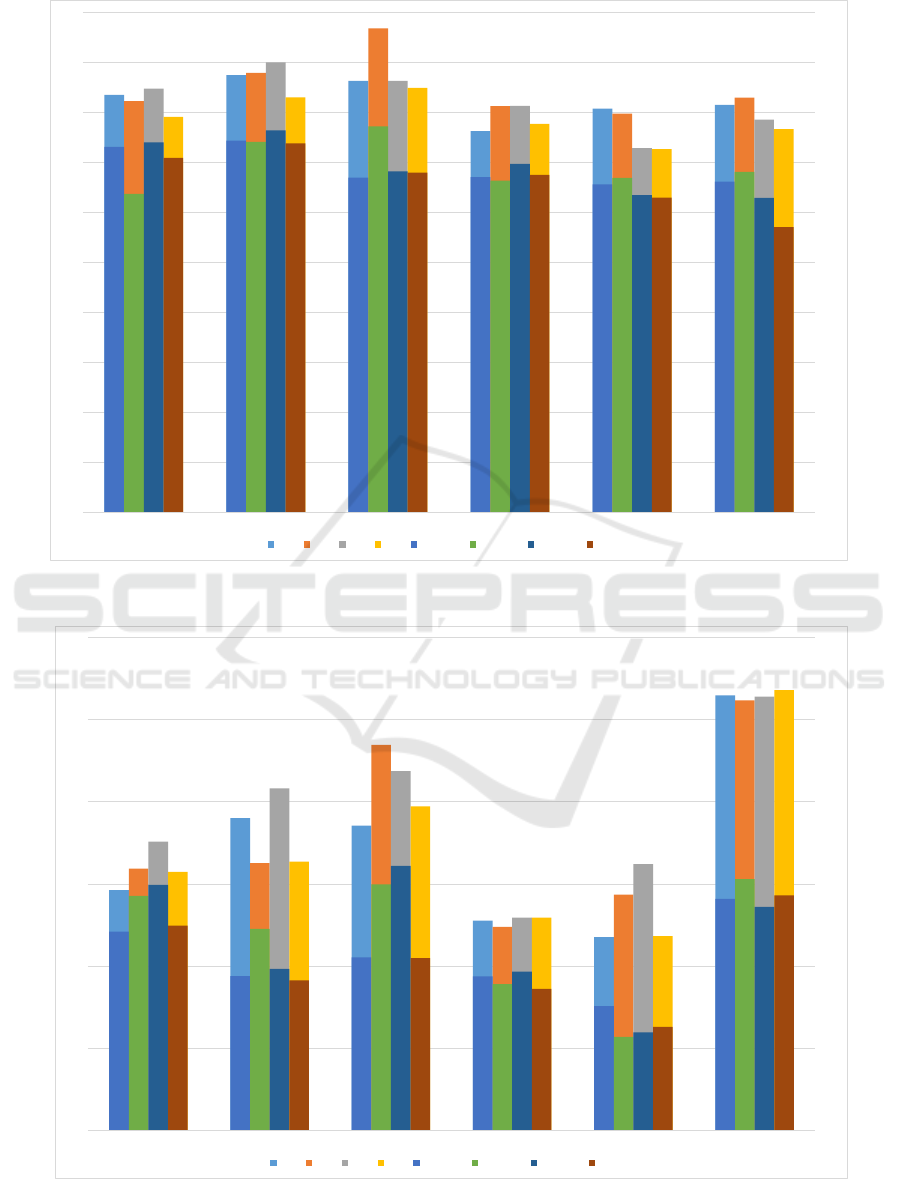
presented in Figure 1. These are the best results
of all the variations we tried and averaged over ac-
curacies of five-fold cross validation. We compare
the results of our SAE classifier against previous
work (Senanayake et al., 2016) we have done on the
same dataset using conventional learning algorithms.
While the results from the SAE classifier is not as
good as the conventional classifiers, there are two sig-
nificant advantages: (i) SAE classifier can be used as
an unsupervised feature extractor/subset selector and
(ii) SAE classifier can be used to combine multiple
modalities of data with ease, as extending this work
to include data from different MR modalities is the
ultimate objective. In addition, the same SAE clas-
sifier can be used as a multi-class classifier as well.
Since the best results were obtained using one vs all
classes experiments, we include a better comparison
in the next subsection.
3.2 One vs All Classes
We present the results of one vs all classes for all
four waves in Figure 2. Clearly the accuracy of the
trained models has improved significantly and this
shows how data dependent the SAE classifier is. This
has been noted before in deep learning literature mul-
tiple times; the more the available data, the better
the performance of the model. We then compare the
results obtained with the SAE classifier against our
previous work (Senanayake et al., 2016) in Table 4.
While the results are comparable, conventional ma-
chine learning algorithms outperform the deep learn-
ing classifier. This is due to the smaller sample size
we have, which hinders the deep learning classifier
from reaching its full potential.
In order to improve the performance of SAE clas-
sifier, we created an ensemble of SAE classifiers at the
ICPRAM 2017 - 6th International Conference on Pattern Recognition Applications and Methods
658

83.44
87.36
86.23
76.2
80.67
81.44
82.19
87.8
96.71
81.16
79.68
82.9
84.69
89.91
86.2
81.24
72.77
78.47
79.03
82.92
84.81
77.63
72.61
76.57
87.65
89.11
80.24
80.39
78.68
79.3
76.4
88.81
92.56
79.54
80.19
81.62
88.72
91.61
81.75
83.58
76.09
75.43
84.97
88.49
81.49
80.96
75.5
68.44
0
20
40
60
80
100
120
0
10
20
30
40
50
60
70
80
90
100
CN vs MCI CN vs aMCI CN vs naMCI MCI Subtypes aMCI Subtypes naMCI Subtypes
W1 W2 W3 W4 AUC W1 AUC W2 AUC W3 AUC W4
Figure 1: Accuracy and area under the ROC curve (AUC) for each wave in one vs one experiments.
84.62
89
88.54
82.77
81.76
96.47
85.93
86.27
93.46
82.4
84.35
96.16
87.57
90.81
91.86
82.95
86.2
96.39
85.73
86.36
89.72
82.96
81.83
96.78
84.21
78.8
81.08
78.77
75.15
88.19
88.54
84.54
89.94
77.83
71.41
90.58
89.9
79.68
92.19
79.34
71.94
87.2
84.92
78.29
81
77.24
72.63
88.61
60
70
80
90
100
110
120
70
75
80
85
90
95
100
aMCI sd-aMCI md-aMCI naMCI sd-naMCI md-naMCI
W1 W2 W3 W4 W1 AUC W2 AUC W3 AUC W4 AUC
Figure 2: Accuracy and area under the ROC curve (AUC) for each wave in one vs all experiments.
Deep Learning Approach for Classification of Mild Cognitive Impairment Subtypes
659

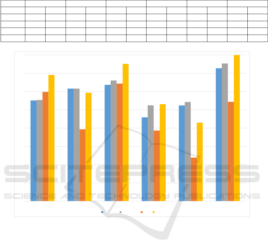
Table 4: Comparison of Deep learning results against previous results for one vs all experiments.
aMCI sd-aMCI md-aMCI naMCI sd-naMCI md-naMCI
SAE Old SAE Old SAE Old SAE Old SAE Old SAE Old
Wave 1 84.62 95.17 89 90.91 88.54 91.88 82.77 88.14 81.76 86.91 96.47 96.96
Wave 2 85.93 95.95 86.27 89.69 93.46 93.15 82.4 87.79 84.35 87.69 96.16 96.83
Wave 3 87.57 97.29 90.81 92.1 91.86 93.05 82.95 88.39 86.2 88.78 96.39 97.07
Wave 4 85.73 03.4 86.36 89.45 89.72 92.13 82.96 84.92 81.83 83.96 96.78 95.97
87.57
90.81
91.86
82.95
86.2
96.39
89.9
79.68
92.19
79.34
71.94
87.2
87.71
90.83
93.03
86.23
87.15
97.7
94.56
89.69
97.59
86.55
81.49
100
60
65
70
75
80
85
90
95
100
aMCI sd-aMCI md-aMCI naMCI sd-naMCI md-naMCI
Accuracy Accuracy-E AUC AUC-E
Figure 3: Comparison of best SAE classifier results against SAE Ensemble classifier results for Wave 3. Accuracy-E and
AUC-E stands for the accuracy and AUC of the SAE ensemble classifier.
model level. We used the same training/testing dataset
to train multiple SAE classifiers with different hyper-
parameters and used these classifiers in conjunction
with a voting scheme, to come up with the final class
label. We present a cross-section of the ensemble we
built taking wave 3 as an example, in Figure 3. While
the accuracies have almost always improved, the area
under the ROC curve has significantly benefited from
creating an ensemble of classifiers. This in turn means
that the classifiers we train are more generalizable and
are robust to noise.
4 DISCUSSION
The diagnostic value of neuropsychological features
has been studied previously (Senanayake et al., 2016).
In this paper, we apply a deep learning technique
in order to compare and contrast the performance of
conventional machine learning techniques. To the
best of our knowledge, this is the first study that com-
pares the use of neuropsychological measures with
deep learning techniques in MCI diagnosis. This
is interesting, as SAEs are usually used with multi-
dimensional data such as images, but we trained our
SAE classifier on a uni-dimensional dataset. Multi-
ple classifiers were trained for different subtypes of
MCI, and the SAE classifiers demonstrate compara-
ble performance to that of conventional techniques.
As deep learning is a data intensive approach, we
presume that with more data, the performance of the
classifier could be further improved. This is clearly
demonstrated in one vs all classes as an increase in
ICPRAM 2017 - 6th International Conference on Pattern Recognition Applications and Methods
660

data points almost always resulted in better perfor-
mance.
In order to improve the performance of individ-
ual classifiers, we have proposed an ensemble of
SAE classifiers that has increased the performance of
the classification task. The proposed ensemble is a
model level ensemble rather than a data level ensem-
ble, as we train different models with different hyper-
parameters on the same training set and test on the
same test set. The results of individual SAE classifiers
are then taken into consideration and the majority vote
is considered as the predicted class label. This enables
us to use different versions of auto-encoders including
conventional auto-encoders and sparse auto-encoders
together. The optimum configuration of the ensemble
was found using grid search.
We note that there is a degree of circularity in us-
ing neuropsychological measures to differentiate be-
tween MCI subtypes, because the same neuropsycho-
logical measures were used to come up with the initial
clinical classification. This is similar to any labeling
process an expert undertakes and we consider the ini-
tial expert labels as a weak classifier with a dynamic
set of exceptions whenever the panel of experts dis-
agree. Our approach builds on top of this weak clas-
sifier, as the SAE classifier improves coverage by in-
cluding more features than the expert. In addition,
the inherent advantage of using SAE based classifiers
is the ability to eliminate feature extraction and se-
lection processes entirely. This in turn enables us to
use MR images directly with the classifier without ex-
tracting features. Another advantage of using a SAE
based classifier is the ability to fuse data from multi-
ple modalities, which we are currently working on.
In conclusion, we suggest that neuropsychologi-
cal measures can be effectively used to differentiate
between MCI and its subtypes. The proposed SAE
based classifier has significant advantages over a con-
ventional classifier, and enables us to combine data
from multiple modalities in order to train a better di-
agnostic system. We believe our work is a step to-
wards reliable MCI diagnosis using neuropsycholog-
ical measures.
REFERENCES
Albert, M. S., DeKosky, S. T., Dickson, D., Dubois, B.,
Feldman, H. H., Fox, N. C., Gamst, A., Holtz-
man, D. M., Jagust, W. J., Petersen, R. C., Sny-
der, P. J., Carrillo, M. C., Thies, B., and Phelps,
C. H. (2011). The diagnosis of mild cognitive im-
pairment due to Alzheimers disease: Recommenda-
tions from the National Institute on Aging-Alzheimers
Association workgroups on diagnostic guidelines for
Alzheimer’s disease. Alzheimer’s & Dementia: The
Journal of the Alzheimer’s Association, 7(3):270–279.
Alexander, A. L., Lee, J. E., Lazar, M., and Field, A. S.
(2007). Diffusion tensor imaging of the brain. Neu-
rotherapeutics, 4(3):316–329. 17599699[pmid].
Baldi, P. (2012). Autoencoders, Unsupervised Learning,
and Deep Architectures. ICML Unsupervised and
Transfer Learning, pages 37–50.
Ch
´
etelat, G., Landeau, B., Eustache, F., M
´
ezenge, F., Vi-
ader, F., de la Sayette, V., Desgranges, B., and Baron,
J.-C. (2005). Using voxel-based morphometry to map
the structural changes associated with rapid conver-
sion in MCI: a longitudinal MRI study. NeuroImage,
27(4):934–46.
Chua, T. C., Wen, W., Chen, X., Kochan, N., Slavin, M. J.,
Trollor, J. N., Brodaty, H., and Sachdev, P. S. (2009).
Diffusion tensor imaging of the posterior cingulate
is a useful biomarker of mild cognitive impairment.
The American journal of geriatric psychiatry : offi-
cial journal of the American Association for Geriatric
Psychiatry, 17(July):602–613.
Chua, T. C., Wen, W., Slavin, M. J., and Sachdev, P. S.
(2008). Diffusion tensor imaging in mild cognitive
impairment and Alzheimer s disease : a review. Cur-
rent Opinions in Neurology.
Cui, Y., Sachdev, P. S., Lipnicki, D. M., Jin, J. S., Luo,
S., Zhu, W., Kochan, N. a., Reppermund, S., Liu,
T., Trollor, J. N., Brodaty, H., and Wen, W. (2012a).
Predicting the development of mild cognitive impair-
ment: A new use of pattern recognition. NeuroImage,
60(2):894–901.
Cui, Y., Wen, W., Lipnicki, D. M., Beg, M. F., Jin, J. S.,
Luo, S., Zhu, W., Kochan, N. a., Reppermund, S.,
Zhuang, L., Raamana, R., Liu, T., Trollor, J. N., Wang,
L., Brodaty, H., and Sachdev, P. S. (2012b). Auto-
mated detection of amnestic mild cognitive impair-
ment in community-dwelling elderly adults: A com-
bined spatial atrophy and white matter alteration ap-
proach. NeuroImage, 59(2):1209–1217.
Gauthier, S., Reisberg, B., Zaudig, M., Petersen, R. C.,
Ritchie, K., Broich, K., Belleville, S., Brodaty, H.,
Bennett, D., Chertkow, H., Cummings, J. L., de Leon,
M., Feldman, H., Ganguli, M., Hampel, H., Schel-
tens, P., Tierney, M. C., Whitehouse, P., and Winblad,
B. (2006). Mild cognitive impairment. The Lancet,
367(9518):1262 – 1270.
Haller, S., Missonnier, P., Herrmann, F. R., Rodriguez, C.,
Deiber, M.-P., Nguyen, D., Gold, G., Lovblad, K.-O.,
and Giannakopoulos, P. (2013). Individual classifica-
tion of mild cognitive impairment subtypes by support
vector machine analysis of white matter DTI. AJNR.
American journal of neuroradiology, 34(2):283–91.
Hedden, T. and Gabrieli, J. D. E. (2004). Insights into the
ageing mind: a view from cognitive neuroscience. Nat
Rev Neurosci, 5(2):87–96.
Hindmarch, I., Lehfeld, H., de Jongh, P., and Erzigkeit, H.
(1998). The bayer activities of daily living scale (b-
adl). Dementia and Geriatric Cognitive Disorders,
9(suppl 2)(Suppl. 2):20–26.
Hinrichs, C., Singh, V., Xu, G., and Johnson, S. C. (2011).
Deep Learning Approach for Classification of Mild Cognitive Impairment Subtypes
661

Predictive markers for AD in a multi-modality frame-
work: An analysis of MCI progression in the ADNI
population. NeuroImage, 55(2):574–589.
Hinton, G. E., Osindero, S., and Teh, Y.-W. (2006). A
Fast Learning Algorithm for Deep Belief Nets. Neural
Computation, 18(7):1527–1554.
Kallenberg, M., Petersen, K., Nielsen, M., Ng, A. Y., Diao,
P., Igel, C., Vachon, C. M., Holland, K., Winkel, R. R.,
Karssemeijer, N., and Lillholm, M. (2016). Unsuper-
vised Deep Learning Applied to Breast Density Seg-
mentation and Mammographic Risk Scoring. IEEE
Transactions on Medical Imaging, 35(5):1322–1331.
Kochan, N. A., Slavin, M. J., Brodaty, H., Crawford, J. D.,
Trollor, J. N., Draper, B., and Sachdev, P. S. (2010).
Effect of Different Impairment Criteria on Prevalence
of &#x201c;Objective&#x201d; Mild Cognitive Im-
pairment in a Community Sample. The American
Journal of Geriatric Psychiatry, 18(8):711–722.
Lemos, L., Silva, D., Guerreiro, M., Santana, I., de Men-
dona, A., Toms, P., and Madeira, S. C. (2012). Dis-
criminating alzheimers disease from mild cognitive
impairment using neuropsychological data. KDD
2012.
Li, F., Tran, L., Thung, K.-H., Ji, S., Shen, D., and Li, J.
(2014). Robust Deep Learning for Improved Classi-
fication of AD/MCI Patients. Machine Learning in
Medical Imaging, 8679:240–247.
Liu, S., Liu, S., Cai, W., Pujol, S., Kikinis, R., and Feng, D.
(2014). Early diagnosis of Alzheimer’s disease with
deep learning. 2014 IEEE 11th International Sym-
posium on Biomedical Imaging (ISBI), pages 1015–
1018.
Mitchell, A. J. and Shiri-Feshki, M. (2009). Rate of pro-
gression of mild cognitive impairment to dementia
meta-analysis of 41 robust inception cohort studies.
Acta Psychiatrica Scandinavica, 119(4):252–265.
Petersen, R. C., Knopman, D. S., Boeve, B. F., Geda, Y. E.,
Ivnik, R. J., Smith, G. E., Roberts, R. O., and Jack,
C. R. (2009). Mild Cognitive Impairment: Ten Years
Later. Archives of neurology, 66(12):1447–1455.
Raamana, P. R., Wen, W., Kochan, N. a., Brodaty, H.,
Sachdev, P. S., Wang, L., and Beg, M. F. (2014). The
sub-classification of amnestic mild cognitive impair-
ment using MRI-based cortical thickness measures.
Frontiers in Neurology, pages 1–10.
Reddy, P., Kochan, N., Brodaty, H., Sachdev, P., Wang, L.,
Beg, M. F., and Wen, W. (2013). Novel ThickNet fea-
tures for the discrimination of amnestic MCI subtypes.
NeuroImage Clinical, 6:284–295.
Reppermund, S., Zhuang, L., Wen, W., Slavin, M. J.,
Trollor, J. N., Brodaty, H., and Sachdev, P. S.
(2014). White matter integrity and late-life depression
in community-dwelling individuals: diffusion tensor
imaging study using tract-based spatial statistics. The
British Journal of Psychiatry, 205:315–320.
Sachdev, P. S., Brodaty, H., Reppermund, S., Kochan,
N. A., Trollor, J. N., Draper, B., Slavin, M. J., Craw-
ford, J., Kang, K., Broe, G. A., Mather, K. A., and
Lux, O. (2010). The sydney memory and ageing study
(mas): methodology and baseline medical and neu-
ropsychiatric characteristics of an elderly epidemio-
logical non-demented cohort of australians aged 7090
years. International Psychogeriatrics, 22:1248–1264.
Sachdev, P. S., Lipnicki, D. M., Crawford, J., Reppermund,
S., Kochan, N. a., Trollor, J. N., Wen, W., Draper,
B., Slavin, M. J., Kang, K., Lux, O., Mather, K. a.,
Brodaty, H., and Team, A. S. (2013a). Factors Pre-
dicting Reversion from Mild Cognitive Impairment to
Normal Cognitive Functioning: A Population-Based
Study. PLoS ONE, 8(3):1–10.
Sachdev, P. S., Zhuang, L., Braidy, N., and Wen, W.
(2013b). Is Alzheimer’s a disease of the white mat-
ter? Curr Opin Psychiatry, 26(3):244–251.
Schmidhuber, J. (2014). Deep Learning in Neural Net-
works: An Overview. pages 1–88.
Senanayake, U., Sowmya, A., Dawes, L., Kochan, N. A.,
Wen, W., and Sachdev, P. (2016). Classification of
mild cognitive impairment subtypes using neuropsy-
chological data. In Proceedings of the 5th Interna-
tional Conference on Pattern Recognition Applica-
tions and Methods, pages 620–629.
Suk, H. I. and Shen, D. (2013). Deep learning-based fea-
ture representation for AD/MCI classification. Lecture
Notes in Computer Science (including subseries Lec-
ture Notes in Artificial Intelligence and Lecture Notes
in Bioinformatics), 8150 LNCS(0 2):583–590.
Thillainadesan, S., Wen, W., Zhuang, L., Crawford, J.,
Kochan, N., Reppermund, S., Slavin, M., Trollor, J.,
Brodaty, H., and Sachdev, P. (2012). Changes in
mild cognitive impairment and its subtypes as seen on
diffusion tensor imaging. International Psychogeri-
atrics, 24:1483–1493.
Winblad, B., Palmer, K., Kivipelto, M., Jelic, V.,
Fratiglioni, L., Wahlund, L.-O., Nordberg, A., Bck-
man, L., Albert, M., Almkvist, O., Arai, H., Basun,
H., Blennow, K., De Leon, M., DeCarli, C., Erkin-
juntti, T., Giacobini, E., Graff, C., Hardy, J., Jack, C.,
Jorm, A., Ritchie, K., Van Duijn, C., Visser, P., and
Petersen, R. (2004). Mild cognitive impairment be-
yond controversies, towards a consensus: report of the
international working group on mild cognitive impair-
ment. Journal of Internal Medicine, 256(3):240–246.
ICPRAM 2017 - 6th International Conference on Pattern Recognition Applications and Methods
662