
Data Clustering Method based on Mixed Similarity Measures
Doaa S. Ali, Ayman Ghoneim and Mohamed Saleh
Department of Operations Research and Decision Support,
Faculty of Computers and Information, Cairo University
5 Dr. Ahmed Zewail Street, Orman, 12613 Giza, Egypt
Keywords: Mixed Datasets, Similarity Measures, Data Clustering Algorithms, Differential Evolution.
Abstract: Data clustering aims to organize data and concisely summarize it according to cluster prototypes. There are
different types of data (e.g., ordinal, nominal, binary, continuous), and each has an appropriate similarity
measure. However when dealing with mixed data set (i.e., a dataset that contains at least two types of data.),
clustering methods use a unified similarity measure. In this study, we propose a novel clustering method for
mixed datasets. The proposed mixed similarity measure (MSM) method uses a specific similarity measure
for each type of data attribute. When computing distances and updating clusters’ centers, the MSM method
merges between the advantages of k-modes and K-means algorithms. The proposed MSM method is tested
using benchmark real life datasets obtained from the UCI Machine Learning Repository. The MSM method
performance is compared against other similarity methods whether in a non-evolutionary clustering setting
or an evolutionary clustering setting (using differential evolution). Based on the experimental results, the
MSM method proved its efficiency in dealing with mixed datasets, and achieved significant improvement in
the clustering performance in 80% of the tested datasets in the non-evolutionary clustering setting and in
90% of the tested datasets in the evolutionary clustering setting. The time and space complexity of our
proposed method is analyzed, and the comparison with the other methods demonstrates the effectiveness of
our method.
1 INTRODUCTION
Unsupervised clustering aims to extract the natural
partitions in a dataset without a priori class
information. It groups the dataset observations into
clusters where observations within a cluster are more
similar to each other than observations in other
clusters (Bhagat et al., 2013; Tiwari and
Jha, 2012).
The K-means clustering algorithm is efficiently used
when processing numerical datasets, where means
serve as centers/centroids of the data clusters. In the
K-means algorithm, observations are partitioned into
K clusters where an observation belongs to the
cluster with the closest mean (i.e., centroid)
(Serapião et al., 2016). When dealing with
categorical data (Bai et al., 2013; Kim, 2008), K-
modes (Ammar and Lingras, 2012) and K-medoids
(Mukhopadhyay and Maulik, 2007) clustering
algorithms are used instead of K-means. In the K-
modes algorithm, modes replace means as the
dissimilarity measure and it uses a frequency based
method to update modes during the clustering
process. On the other hand, K-medoids algorithm
computes a cluster medoid instead of computing the
mean of cluster. A medoid is a representative
observation in a cluster, where the sum of distances
to other observations in the cluster is minimal
(Mukhopadhyay and Maulik, 2007).
There are four main types of data attributes,
which are nominal, ordinal, binary, and numerical.
Ordinal and nominal attributes are used to describe
categorical data. Nominal attributes are used for
labeling variables without any quantitative value.
Nominal attributes are mutually exclusive (no
overlap) and none of them have any numerical
significance such as name, gender, and colors.
Ordinal data attributes have ordered values to
capture importance and significance, but the
differences are not quantified such as (excellent,
very good, good and bad) and (very happy, happy,
and unhappy). Numerical data attributes can be
either discrete or continuous (e.g., temperature,
height and weight). Distance or similarity measures
are used to solve many pattern recognition problems
such as classification, clustering, and retrieval
192
S. Ali D., Ghoneim A. and Saleh M.
Data Clustering Method based on Mixed Similarity Measures.
DOI: 10.5220/0006245601920199
In Proceedings of the 6th International Conference on Operations Research and Enterprise Systems (ICORES 2017), pages 192-199
ISBN: 978-989-758-218-9
Copyright
c
2017 by SCITEPRESS – Science and Technology Publications, Lda. All rights reserved

problems (Cha, 2007). A distance is mathematically
defined as a quantitative degree of how far apart two
data points are. The choice of distance/similarity
measures depends on the type of data attributes in
the processed dataset.
Most of the traditional clustering models are
built to deal with either numerical data or categorical
data. However in the real world, the collected data
often have both numeric and categorical attributes
(i.e., a mixed dataset). Thus it’s hard to apply
traditional clustering algorithm directly to such
mixed datasets. When it comes to dealing with
mixed datasets, previous work adopted two
approaches. The first approach unified the used
similarity measure when dealing with mixed datasets
(e.g., Parameswari et al., 2015; Shih et al., 2010 and
Soundaryadevi and Jayashree, 2015). It converts the
mixed dataset either to pure numerical data or to
pure categorical data using a pre-processing step
before applying the clustering algorithm.
Unfortunately, this approach is not practical because
there are data instances where the conversion does
not give meaningful numerical data. Furthermore,
this conversion may lead to loss of information. The
second approach divides the original dataset into
pure numerical and categorical dataset (e.g. Asadi et
al., 2012; Ahmad, 2007; Shih et al., 2010;
Mutazinda et al., 2015; and Pinisetty et al., 2012).
The appropriate clustering algorithms are used to
produce corresponding clusters for these pure
datasets. The clustering results on the categorical
and numerical datasets are then combined as a
categorical dataset on which a categorical data
clustering algorithm is employed to get the final
output. This approach suffers from excessive
complexity through the implementation, especially
in the case of dealing huge/large dataset.
Recently, researchers have given much attention
to distance learning metric for semi-supervised
clustering algorithms (e.g. Relevant Component
Analysis, Discriminative Component Analysis) at
handling mixed/or complicated datasets (Kumar and
Kummamuru, 2008; Baghshah and Shouraki, 2009).
Semi-supervised learning clustering algorithms
partition a given dataset using additional supervisory
information (Kumar and
Lingras, 2008). The most
popular form of supervision used in this category of
clustering algorithms is in terms of pairwise
constraints. Learning in a distance metric is
equivalent to finding a rescaling of a given dataset
by applying the standard Euclidean metric (Xing,
2003). Distance learning metric is mainly processed
for semi-supervised clustering algorithms and also
suffers from exaggerated complexity through the
implementation.
To overcome the previous limitations, we
introduce a novel clustering method for the mixed
datasets. The proposed mixed similarity measure
(MSM) method uses the appropriate similarity
measure for each type of data attribute. It combines
the capabilities of the K-modes and K-means
algorithms when computing distances and updating
centers for the clusters. The proposed MSM method
is tested using six benchmark real life datasets
obtained from the UCI Machine Learning
Repository (Blake and Merz, 1998), and it achieved
a significant improvement in the clustering
performance in a non-evolutionary clustering setting
and in an evolutionary clustering setting.
The time
and space complexity of our proposed method is
analyzed, and the comparison with the other
methods proves the effectiveness of our method.
The rest of the paper is organized as follows.
Section 2 introduces some related works and a
background to K-means, K-modes algorithms, and
differential evolution. Section 3 presents the
proposed MSM method. Section 4 illustrates the
differential evolution MSM setting. Section shows
the experimental results and analyses. Section 6
concludes the work and discusses future works.
2 BACKGROUND
In this section, we cover preliminary concepts
needed in our work. These preliminary concepts are
the clustering problem, K-means and K-modes
clustering algorithms, and differential evolution
algorithm.
2.1 Clustering Problem
Formally, a clustering problem is represented as an
optimization problem as follows:
,
μ,
,
1, 1
1
where n is the number of data points, k is the
number of data clusters, and µ
ij
is a membership of
i
th
data observation to cluster j (i.e.
takes binary
values in crisp case).
,
is the matching
distance measure between data point x
i
and data
cluster center z
j .
Data Clustering Method based on Mixed Similarity Measures
193

2.2 K-Means Clustering Algorithm
The K-means algorithm is a widely used clustering
algorithm for numerical data sets because of its
simplicity (Bai et al., 2013). K-means algorithm
searches for nearly optimal partitions with a fixed
number of clusters. The algorithm aims to minimize
total distances between data points and centers (Wu
et al., 2008) where
,
(2)
is the distance measure between data point x
i
and
data cluster center z
j
. The steps of K-means
clustering algorithm are as follows (Kim and
Hyunchul, 2008):
1:
Randomly initialize centers for the k clusters
2:
Each data point is assigned to the cluster with the nearest
center (Eq. 2).
3:
Update the center of each cluster.
4:
Repeat steps 2 and 3 until the clusters’ centers stop changing
or other stopping criteria are met.
Procedure 1: Steps of K-Means algorithm.
In step 3, the j
th
cluster center is updated by
taking the mean of data observations which are
grouped in cluster j in step 2.
2.3 K-Modes Clustering Algorithm
K-modes clustering algorithm extends the K-means
algorithm to cluster categorical data (Gibson et al.,
1998), by replacing means of clusters by modes. K-
modes algorithm uses a simple matching distance
(Aranganayagi and
Thangavel
, 2009), or a hamming
distance when measuring distances between data
observations. To understand the matching distance
measure, let x and y be two data observations in D
dataset and L be the number of attributes in a data
observation. The simple matching distance measure
between x and y in D is defined as:
,
,
(3)
where
,
0
1
.
The steps of the k-modes clustering algorithm is
similar to the k-means algorithm (Procedure 1),
except that the center of cluster is updated according
to the following equation:
∈
, ∈
(4)
where
represents the new updated value of cluster
j in the
attribute, and
is the value of the data
observation r which has the most frequent value in
the
attribute for the data observations within
cluster j. With respect to
, it expresses all the
possible values which can be taken by the attribute
and DOM is a domain of this attribute.
is the
total number of data observations in cluster j.
2.4 Differential Evolution
Differential evolution (DE) is a population-based
global optimization algorithm that uses a real-coded
representation (Saha et al., 2010). DE belongs to the
class of genetic algorithms since it uses selection,
crossover, and mutation operators to optimize an
objective function over the course of successive
generations (Suresh et al., 2009). The DE operators
are as follow:
1. Mutation operator: In generation t, let
,
be the
i
th
solution vector in the population of size NP
(i.e., ∈1,2,…,). For each solution vector
,
, a mutant vector
,
is generated using three
randomly picked solutions from the population
using the following equation:
,
,
,
,
(5)
where
,
,
∈1,2,…, are three mutually
distinct random numbers and
,
,
, and
∈0,2 is a real number representing the
differential weight.
2. Crossover operator: Let L be the dimension of a
solution vector and 1,2,…, be the index for
the dimension. The mutant vector
,
and the
target solution vector
,
are crossed to generate a
trial solution vector
,
,
,
,
,…,
,
(6)
where
,
,
,
,
,
,
.
where
∈
0,1
is a uniformly generated random
number, ∈
0,1
is the crossover probability,
and
∈1,2,…, is a randomly chosen
dimension index.
3. Selection operator: The trail vector
,
is
compared against
,
and will replace it in the
population if the following condition is met where
.
is the fitness function:
,
,
,
,
,
,
, .
(7)
ICORES 2017 - 6th International Conference on Operations Research and Enterprise Systems
194
3 MSM METHOD
The proposed MSM method is a novel clustering
model based on using different similarity measures
when dealing with mixed datasets. The MSM
method has a pool of different similarity measures
and uses them according to the type of data attribute
under consideration. When computing distances and
updating centroids, the MSM method merges
between the capabilities of k-modes and K-means
algorithms. Thus, we modify some steps in the
traditional clustering model. Procedure 2 shows the
steps of the MSM method. These modified steps are
explained in details in the next sub-sections.
1:
All data elements are assigned a cluster number between 1
and k randomly, where k is the number of clusters desired.
2:
Find the cluster center of each cluster.
3:
For each data element, find the cluster center that is closest
to the element. Assign the element to the cluster whose
center is closest to it.
4:
Re-compute the cluster centers with the new assignment of
elements.
5:
Repeat steps 3 and 4 till clusters do not change or for a
fixed number of times.
Procedure 2: Steps of the MSM method.
3.1 Computing Distances
In the proposed MSM method, let A and B be two
mixed data points with m attributes. When
computing the distance between A and B, the MSM
method calls the similarity measure according to the
attribute type, and compute a sub-distance between
the attribute in A and the same attribute in B. The
total distance between A and B is the sum of the
sub-distances for the m attributes. The used
similarity measures are normalized to be in the [0, 1]
interval as follows:
For ordinal data attribute
,
,
1
(8)
where z
,
isthe standarized value of attribute
a
of the data object i, r
,
isthedifference
value before standardization, M
is the upper
limit of the domain of attribute a
.
For binary and nominal data attribute, we use the
matching distance (Equation 3).
For numerical data attribute, we use the
following equation
zijn
,
,
max
min
(9)
where z
,
is the standardized difference value
of attribute a
between two data objects i and
j, x
,
andx
,
are the values of attribute a
of
object i and j before standardization, max x
n
and min x
n
are the upper and lower limit of the
domain of attribute a
, respectively.
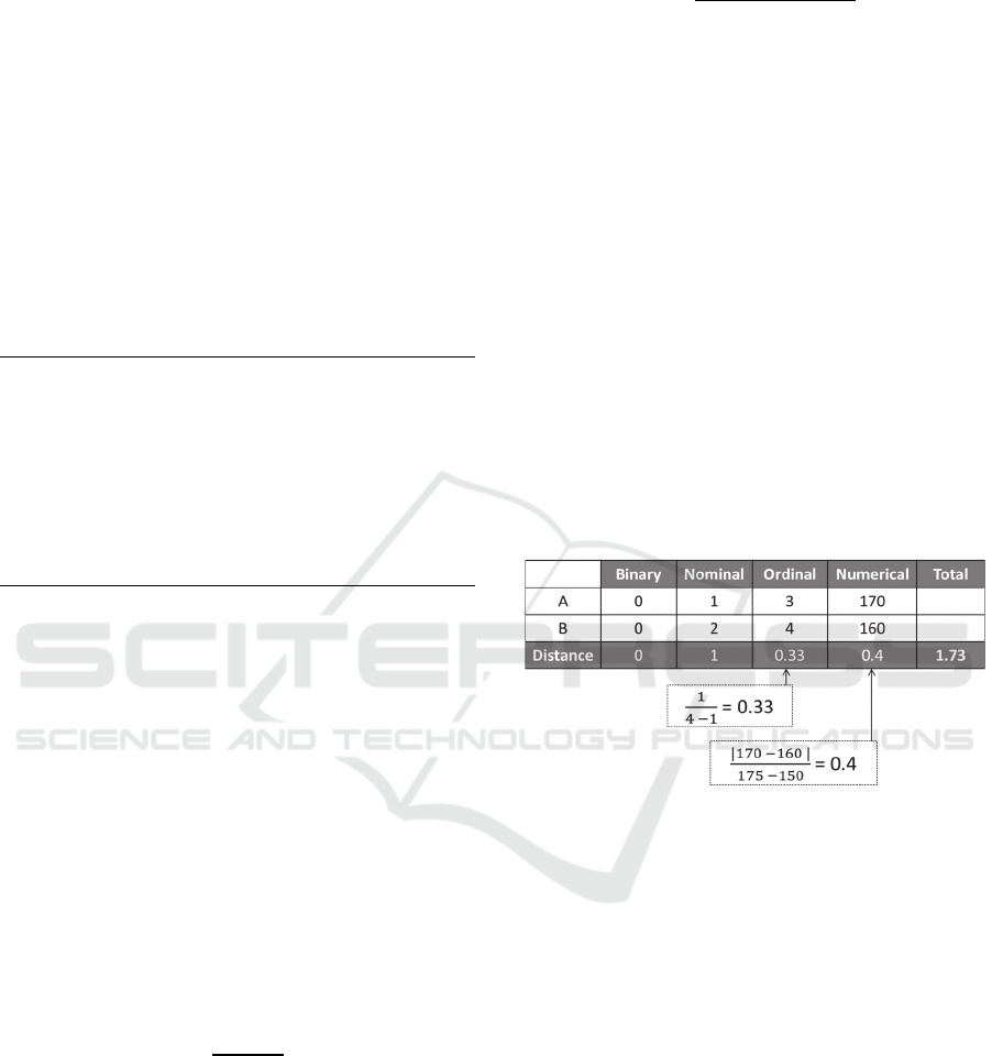
Figure 1 shows an example of two mixed data
points A and B. The first two attributes are
binary and nominal, so the matching distance
is used in measuring the distance between
them. The third attribute is ordinal, so the sub-
distance is calculated using equation 4, where
the domain of this attribute is from 1 to 4. The
last attribute is numerical and has the range
[150, 175], so the sub-distance is calculated by
equation 6. Finally, the total distance between
A and B is the sum of these sub-distances,
which will be 1.73.
Figure 1: An example of calculating the distances in the
MSM method.
3.2 Updating Centers
Generally speaking, the step of updating centers
differs according to the type of data (e.g., categorical
or numerical). Thus when updating centers, the
proposed MSM method updates each value of
attribute according also to the data type (see Figure
2). If the value of attribute is numerical, then we use
the updating rule of the k-means algorithm.
However if the value of attribute is categorical, then
we use the updating rule of the k-modes algorithm.
Data Clustering Method based on Mixed Similarity Measures
195
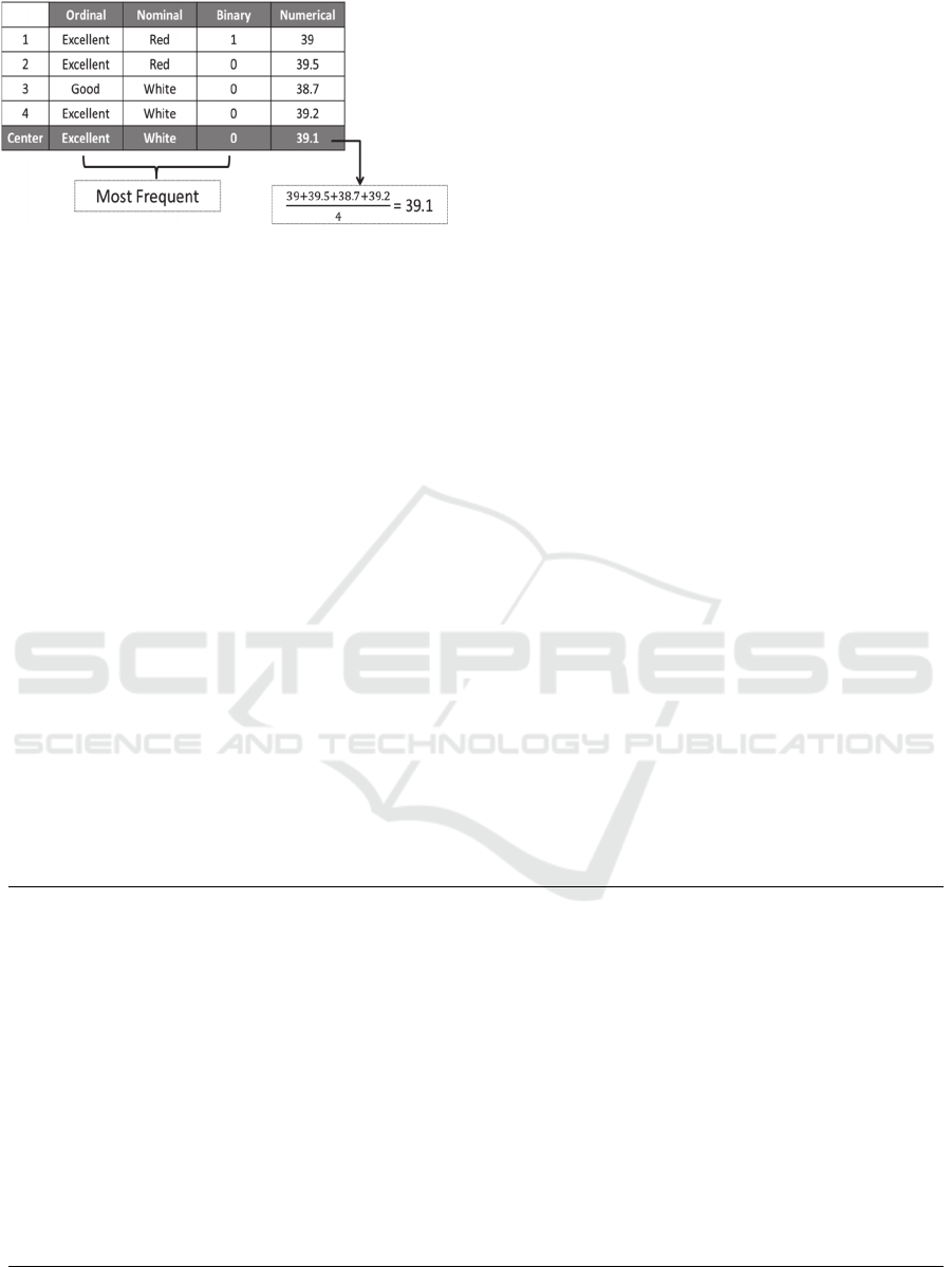
Figure 2: Example for updating centers in the MSM
method.
4 EXPERIMENTAL DESIGN
Measuring similarity between data points is a corner
stone in the clustering process, whether it is a non-
evolutionary clustering setting (e.g., Procedures 1
and 2) or in an evolutionary clustering setting. Thus
to evaluate the performance of the MSM method, we
compared it against other existing similarity
measures in (Boriah et al., 2008) (i.e., matching
distance, IOF, and Eskin similarity measures) in
addition to the scaling method in (Parameswari et
al., 2015) assuming both the non-evolutionary and
evolutionary settings. Evolutionary computation
techniques play a vital role in improving the data
clustering performance because of its ability to avoid
falling in local optimal solutions.
We use differential evolution (DE) as an
evolutionary technique, where a similarity measure
becomes a sub-routine used within the evolutionary
setting. For DE with the MSM method (denoted by
DE-MSM), procedure 3 illustrates the steps of the
algorithm. In step 3, the initialized centers of
clusters are randomly determined. The next steps
represent the main part of the proposed method,
where it starts with updating centers, then updating
distances. The mutation and crossover operators then
have to be applied using Equations 5 and 6,
respectively. The resulting new individual is a
candidate which is evaluated against its parent using
Equation 7 to select the one with the better fitness.
When reaching the maximum number of iterations,
we use the accuracy measure performance (Arbelaitz
et al., 2013) to select the best individual of the final
population.
For the DE, we use a population size of 100
individuals (i.e., 100 different sets of centers),
maximum number of iterations of 100, and
crossover rate CR of 0.2. These parameters are
chosen based on preliminary experiments.
5 EXPERIMENTAL RESULTS
AND DISCUSSIONS
The proposed method is tested on six real-life mixed
datasets obtained from the UCI Machine Learning
Repository (Blake and Merz, 1998). The obtained
results of 100 independent runs are summarized in
table 1 for the non-evolutionary setting. Table 1
contains the mean and standard deviation of best
result of accuracy. We compare the MSM method
against three similarity measures(i.e., matching
distance, IOF, Eskin, and Scaling) already existing
in the literature. We performed T-test with
1:
Input: D = the used dataset, K = number of data clusters, NP = population size
2:
Output: clusters assignment
3:
Add randomly initialized clusters’’ centers (i.e., individuals of population).
4:
Evaluate the fitness of all individuals.
5:
While Stopping Criterion (i.e., maximum number of iterations) is not met; do:
6:
For each Individual Pi (i = 1 … NP) in the population, do:
7:
a) Update centers of the k clusters.
8:
b) Update distance between data objects and the updated centers of clusters.
9:
c) Apply the mutation operator using Eq. 5.
10:
d) Apply the crossover using Eq. 6.
11:
e) Evaluate the fitness of the offspring C from parent Pi.
12:
f) Apply selection operator to create new-population by comparing the offspring C against its parent Pi using Eq. 7.
13:
End For
14:
End While
15:
Calculate the accuracy measure performance for every individual in the final population.
16:
Select the best solution (i.e., set of centers) which has the highest accuracy.
Procedure 3: The DE-MSM method.
ICORES 2017 - 6th International Conference on Operations Research and Enterprise Systems
196

Table 1: Mean ± standard deviation of best solution of 100 independent runs for the simple matching, IOF, Eskin, Scaling
and the proposed MSM method.
Simple
Matching
IOF Eskin Scaling MSM T-test
Breast Cancer 0.8128434 ±
2.69461E-06
0.771992 ±
0.001752535
0.782972 ±
0.001451745
0.814782 ±
0.0027383
0.839089 ±
6.0179E-06
Significant
Zoo 0.8787367 ±
0.000736404
0.861041 ±
0.000184208
0.880504 ±
0.00144237
0.885224 ±
0.0056389
0.913004 ±
0.000432323
Significant
Hepatitis 0.766462 ±
0.000562314
0.710596 ±
0.003786261
0.669242 ±
0.00143719
0.769892 ±
0.0056282
0.8187971 ±
2.72221E-05
Significant
Heart Diseases 0.7520178 ±
9.35633E-06
0.778464 ±
0.001182946
0.6315967 ±
0.000205821
0.761143 ±
0.00088239
0.7953947 ±
1.06071E-05
Significant
Dermatology 0.8476637 ±
0.00152124
0.699989 ±
0.00055469
0.6957118 ±
0.000270416
0.856321 ±
0.0003345
0.8424427 ±
3.90709E-05
Significant
Credit 0.9043666 ±
4.05246E-06
0.864447 ±
0.003066162
0.6360959 ±
0.001083251
0.91882 ±
0.0004267
0.8960072 ±
1.21558E-05
Significant
confidence level 0.05 to illustrate the statistical
significant of the results obtained by the MSM
method and the second best similarity measure. As
shown in Table 1, the MSM method obtained
statistically significant better results for four
datasets, while simple matching obtained better
results for two datasets (where one is not statistically
significant). Based on the results, the proposed
MSM methods performed better when compared
with the other similarity methods, and it improved in
about 80% of the tested datasets. Moreover, Table 2
lists the run time of the five clustering similarity
methods on different datasets. From Table 2, we can
see that the MSM method needs more time than the
simple matching method. However, the MSM
method consumes time less than IOF, Eskin, and
Scaling methods.
Table 2: The running time of the five clustering models on
the used datasets.
Average Running Time (Minutes)
Simple
Matching
IOF Eskin Scaling MSM
Breast
Cancer
4.82 5.33 5.47 4.97 4.94
Zoo 2.11 2.26 2.34 2.17 2.10
Hepatitis 2.69 3.24 3.32 2.87 2.63
Heart
Diseases
3.17 3.38 3.41 3.27 3.22
Dermatology 3.68 3.87 3.96 3.71 3.72
Credit 5.19 5.42 5.49 5.34 5.21
We now move to the evolutionary clustering
setting, where each similarity measure is used as a
sub-routine to compute distances and update centers
in the DE algorithm. For the same six real-life mixed
datasets, the obtained results of the 100 independent
runs are reported in Table 3. Table 3 contains the
mean and standard deviation of best result of the
accuracy measure performance. To compare our
results, we compared the DE with different
similarity measures (i.e., DE-MSM, DE-Simple
matching, DE-IOF, DE-Eskin,
DE-Scaling). Based
on the experimental results, the DE setting (Table 3)
yields higher accuracy compared to the non-
evolutionary setting (Table 1). In addition as shown
in Table 3, the DE-MSM obtained statistically
significant better results for five datasets, while
simple matching obtained better results for one
dataset.
6 CONCLUSION AND FUTURE
WORK
In this study, we proposed a novel clustering MSM
method for the mixed datasets (i.e., datasets with at
least two types of data attributes). In contrast to
existing approaches in literature dealing with mixed
datasets, the MSM method assigns a unique
similarity measure for each type of data attribute
(e.g., ordinal, nominal, binary, continuous). When
dealing with a pure dataset (i.e., with only one type
of data attributes), the MSM method will reduce to
the K-means or the K-modes algorithms. Using six
benchmark real life mixed datasets from the UCI
Machine Learning Repository, we first compared the
performance of the MSM method against other
similarity measures (i.e., simple matching, IOF,
Eskin, and Scaling) in a non-evolutionary setting.
Data Clustering Method based on Mixed Similarity Measures
197

Table 3: Mean ± standard deviation of best solution of 100 independent runs for the DE-simple matching, DE-IOF, DE-
Eskin, DE-Scaling, and DE-MSM.
DE-Simple
Matching
DE-IOF DE-Eskin DE-Scaling DE-MSM T-test
Breast Cancer
0.823201 ±
00013254
0.7901874 ±
0.000231
0.805437 ±
0.006119
0.82289 ±
000245
0.8472614 ±
0.07811E-05
Significant
Zoo
0.90132 ±
0.0002621
0.884791±
0.6119E-04
0.899645 ±
0.00332
0.908892 ±
0.002583
0.9435833 ±
2.52812 E-06
Significant
Hepatitis
0.798517±
0.003213
0.769026 ±
0.00371
0.734618 ±
1.842E-04
0.797582±
0.0007739
0.83306326 ±
7.2235E-05
Significant
Heart
Diseases
0.762825 ±
0.000765
0.7356806 ±
2.5723E-05
0.6571352 ±
0.00422
0.774329 ±
0.000113
0.82840165 ±
3.77392E-05
Significant
Dermatology
0.85060403
± 0.000113
0.7285605 ±
0.00117
0.705437 ±
0.0005632
0.8505721 ±
0.00017
0.86351823 ±
1.4426 E-04
Significant
Credit
0.9392598 ±
0.0006234
0.88369739
± 0.000921
0.7401278 ±
3.48192E-04
0.940456 ±
0.000253
0.91358951 ±
0.000218
Significant
The experimental results showed that the MSM
method achieved statistically significant accuracy in
80% of the tested datasets. We then move to
evolutionary setting using DE where similarity
measures were used to compute distance and update
centers during the search process. DE showed its
ability to improve the clustering performance
compared to the non-evolutionary setting, and DE-
MSM achieved statistically significant accuracy in
90% of the tested datasets compared to DE-simple
matching, DE-IOF, DE-Eskin and DE-Scaling. The
time and space complexity of our proposed method
is analyzed, and the comparison with the other
methods confirms the effectiveness of our method.
For future work, the proposed MSM and/or DE-
MSM methods can be used in a multiobjective data
clustering framework to deal specifically with mixed
datasets. Furthermore, the current work can be
extended to data clustering models with uncertainty.
REFERENCES
Ahmad, Dey L., 2007, A k-mean clustering algorithm for
mixed numeric and categorical data, Data &
Knowledge Engineering, 63, pp. 503–527.
Ammar E. Z., Lingras P., 2012, K-modes clustering using
possibilistic membership, IPMU 2012, Part III, CCIS
299, pp. 596–605.
Aranganayagi S., Thangavel K., 2009, Improved K-
modes for categorical clustering using weighted
dissimilarity measure, International Journal of
Computer, Electrical, Automation, Control and
Information Engineering, 3 (3), pp. 729–735.
Arbelaitz O., Gurrutxaga I., Muguerza J., Rez J. M.,
Perona I., 2013, An extensive comparative study of
cluster validity indices, Pattern Recognition (46), pp.
243–256.
Asadi S., Rao S., Kishore C., Raju Sh., 2012, Clustering
the mixed numerical and categorical datasets using
similarity weight and filter method, International
Journal of Computer Science, Information Technology
and Management, 1 (1-2).
Baghshah M. S., Shouraki S. B., 2009, Semi-supervised
metric learning using pairwise constraints,
Proceedings of the Twenty-First International Joint
Conference on Artificial Intelligence (IJCAI), pp.
1217–1222.
Bai L., Lianga J., Dang Ch., Cao F., 2013, A novel fuzzy
clustering algorithm with between-cluster information
for categorical data, Fuzzy Sets and Systems, 215, pp.
55–73.
Bai L., Liang J., Sui Ch., Dang Ch., 2013, Fast global k-
means clustering based on local geometrical
information, Information Sciences, 245, pp. 168-180.
Bhagat P. M., Halgaonkar P. S., Wadhai V. M., 2013,
Review of clustering algorithm for categorical data,
International Journal of Engineering and Advanced
Technology, 3 (2).
Blake, C., Merz, C., 1998. UCI repository machine
learning datasets.
Boriah Sh., Chandola V., Kumar V., 2008, Similarity
measures for categorical data: A comparative
evaluation. The Eighth SIAM International
Conference on Data Mining. pp. 243–254.
Cha S., 2007, Comprehensive survey on
distance/similarity measures between probability
density functions, International journal of
mathematical models and methods in applied sciences,
1(4), pp. 300–307.
Gibson D., Kleinberg J., Raghavan P., 1998, Clustering
categorical data: An approach based on dynamical
systems, In 24th International Conference on Very
Large Databases, pp. 311–322.
ICORES 2017 - 6th International Conference on Operations Research and Enterprise Systems
198

Kim K.K., Hyunchul A., 2008, A recommender system
using GA K-means clustering in an online shopping
market, Elsevier Journal, Expert Systems with
Applications 34, pp. 1200–1209.
Kumar N., Kummamuru K., 2008, Semi-supervised
clustering with metric learning using relative
comparisons, IEEE Transactions on Knowledge and
Data Engineering, 20 (4), pp. 496–503.
Mukhopadhyay A., Maulik U., 2007, Multiobjective
approach to categorical data clustering, IEEE
Congress on Evolutionary Computation, pp. 1296 –
1303.
Mutazinda H., Sowjanya M., Mrudula O., 2015, Cluster
ensemble approach for clustering mixed data,
International Journal of Computer Techniques, 2 (5),
pp. 43–51.
Parameswari P., Abdul Samath J., Saranya S., 2015,
Scalable clustering using rank based preprocessing
technique for mixed data sets using enhanced rock
algorithm, African Journal of Basic & Applied
Sciences, 7 (3), pp. 129–136.
Pinisetty V.N. P., Valaboju R., Rao N. R., 2012, Hybrid
algorithm for clustering mixed data sets, IOSR Journal
of Computer Engineering, 6, pp 9–13.
Saha, D. Plewczy´nski, Maulik U., Bandyopadhyay S.,
2010, Consensus multiobjective differential crisp
clustering for categorical data analysis, RSCTC, LNAI
6086, pp. 30–39.
Serapião B. S., Corrêa G. S. , Gonçalves F. B. , Carvalho
V. O., 2016, Combining K-means and K-harmonic
with fish school search algorithm for data clustering
task on graphics processing units, Applied Soft
Computing, 41, pp. 290–304.
Shih M., Jheng J., Lai L., 2010, A two-step method for
clustering mixed categroical and numeric data,
Tamkang Journal of Science and Engineering, 13 (1),
pp. 11–19.
Soundaryadevi M., Jayashree L.S., 2014, Clustering of
data with mixed attributes based on unified similarity
metric, Proceedings of International Conference On
Global Innovations In Computing Technology, pp.
1865–1870.
Suresh K., Kundu D., Ghosh S. , Das S., Han, Y. S., 2009,
Multi-Objective Differential Evolution for Automatic
Clustering with Application to Micro-Array Data
Analysis, Sensors, 9(5), pp. 3981–4004.
Tasdemir K., Merényi E., 2011, A validity index for
prototype-based clustering of data sets with complex
cluster structures, IEEE transactions on systems, man,
and cybernetics—part b, 41(4), pp. 1039–1053.
Tiwari M., Jha M. B., 2012, Enhancing the performance of
data mining algorithm in letter image recognition data,
International Journal of Computer Applications in
Engineering Sciences, II (III), pp. 217–220.
Wu X., Kumar V., Quinlan J. R., Ghosh J., Yang Q. ,
Motoda H., McLachlan G. J., Ng A., Liu B. , Yu Ph.
S., Zhou Zh., Steinbach M., Hand D. J., Steinberg D.,
2008, Top 10 algorithms in data mining, Knowledge
Information System, 14, pp. 1–37.
Xing E., 2003, Distance metric learning with application
to clustering with side-information, in NIPS, pp. 505–
512.
Data Clustering Method based on Mixed Similarity Measures
199
