
A 3D Anti-collision System based on Artificial Potential Field Method for
a Mobile Robot
Carlos Morais, Tiago Nascimento, Alisson Brito and Gabriel Basso
LASER - Embedded Systems and Robotics Lab, Department of Computer Systems, Federal University of Paraiba (UFPB),
Cidade Universit
´
aria, Jo
˜
ao Pessoa PB, Brazil
Keywords:
3D Anti-collision System, Artificial Potential Field, Mobile Robot, Kinect.
Abstract:
Anti-collision systems are based on sensing and estimating the mobile robot pose (coordinates and orientation),
with respect to its environment. Obstacles detection, path planning and pose estimation are primordial to
ensure the autonomy and safety of the robot, in order to reduce the risk of collision with objects and living
beings that share the same space. For this, the use of RGB-D sensors, such as the Microsoft Kinect, has
become popular in the past years, for being relative accurate and low cost sensors. In this work we proposed
a new 3D anti-collision algorithm based on Artificial Potential Field method, that is able to make a mobile
robot pass between closely spaced obstacles, while also minimizing the oscillations during the cross. We
develop our Unmanned Ground Vehicles (UGV) system on a ’Turtlebot 2’ platform, with which we perform
the experiments.
1 INTRODUCTION
Recently, mobile robots have been developed for
many different applications, such as surveillance,
defense, rescue, mobile health care, border con-
trol , agricultural production support, entertainment,
among others. Nonetheless, there are a variety of po-
tential applications still unexploited. One of the main
problems regarding autonomous mobile robot it the
capability to move between obstacles and effectively
avoid collision with them, which itself includes sub-
problems such as object detection, robot tracking and
path planning.
Regarding obstacles detecting in the robot en-
vironment, two different approaches are commonly
adopted: one is to imbue sensors on the robot, in an
embedded detection scheme, and the other is to set
them on the environment itself. The mixed approach
is also possible. For embedded detection, there are a
range of sensors (RGB-D sensors, as the Kinect, cam-
eras, lasers, LiDARs, sonars, etc.) suitable to give the
robot some perspective of the environment. Another
important issue for autonomous robot is tracking the
robots own position in space, over time. This is fun-
damentally necessary, because the robot must know
what is its current pose in order to estimate the dis-
tance from its target, and the correct path to it. That
is achieved with embedded detection scheme through
the use of dead reckoning methods, such as getting
the encoder data or the Kinect data (visual odometry)
(Scaramuzza and Fraundorfer, 2011).
Many different methods to avoid collision, in con-
junction with path planning, are explored in the liter-
ature, such as tangential escape (Santos et al., 2015),
corner detection (Borenstein and Koren, 1988), oc-
cupation grid (Elfes, 1987), artificial potential field
(Hwang and Ahuja, 1992; Tan et al., 2010; Nasci-
mento et al., 2014; Mac et al., 2016), and Virtual
Force and Virtual Field (Elfes, 1987).
Specifically, the potential field method (PFM) is
an interesting way to avoid collision, being relatively
simple to implement, efficient, fast and accurate for
most applications. However, the traditional PFM is
usually subject to problems with local minimums in
the potential field, which generate limitations such as:
1. No passage between closely spaced obstacles.
2. Oscillations in the presence of obstacles.
3. Oscillations in narrow passages.
4. Non-reachable target.
This work presents a 3D anti-collision system that
uses a new modified artificial potential field method,
that solves three typical problems of the PFM:
1. Solution of the ”no passage between closely
spaced obstacles” problem;
308
Morais C., Nascimento T., Brito A. and Basso G.
A 3D Anti-collision System based on Artificial Potential Field Method for a Mobile Robot.
DOI: 10.5220/0006245303080313
In Proceedings of the 9th International Conference on Agents and Artificial Intelligence (ICAART 2017), pages 308-313
ISBN: 978-989-758-219-6
Copyright
c
2017 by SCITEPRESS – Science and Technology Publications, Lda. All rights reserved

2. Solution of the ”oscillations in the presence of ob-
stacles” problem;
3. Solution of the ”oscillations in narrow passages”
problem.
We implemented our technique, tested our al-
gorithms and performed the experiments on a mo-
bile robot called ’Turtlebot 2’, which is a low cost
platform used to develop academics researches, and
whose encoders and compass allow us to get an es-
timation of its displacement over time through the
dead reckoning method (Scaramuzza and Fraundor-
fer, 2011). The obstacle detection was done via vi-
sual information, captured through the RGB-D Kinect
sensor and processed to 3D images via Point Cloud
Library (PCL). The voxelgrid and passtrough filters
enables us to optimize the computation, reducing
computational costs, and specify the dimensions of
interest, respectively.
The next session introduces the related works,
then the proposed new artificial potential field
method, our experiments realized with the Turtlebot
and finally, the conclusions.
2 RELATED WORKS
To avoid collisions, Tarazona (Fonnegra Tarazona
et al., 2014) presents an anti-collision system for a
unmanned aerial vehicle (UAV) able to navigate in-
door using a Fuzzy controller. Santos (Santos et al.,
2015) proposed a case study of an anti-collision strat-
egy based on a tangential escape approach, where the
UAV can take one of the following ways to escape:
lateral or vertical tangents.
Elfes (Elfes, 1987) shows a method called ”occu-
pation grid”, that breaks the observable region in cells
(in a cone-shape, in front of the sensor) and then com-
putes the probability of each cell being occupied or
not (with an obstacle). For such, it used sonars to pro-
duce a bi-dimensional map of the environment and
assist the robot navigation. Souza (Souza and Maia,
2013) presents an approach based on a stereo system
(two cameras) that generates a 3D occupation grid,
taking into account the obstacle elevation, which is
able to interfere on the decision of the mobile robot to
continue to drive through this same obstacle or not.
Another approach, proposed by Hwang (Hwang
and Ahuja, 1992), attributes a potential function to
each obstacle to identify the chance of a collision
with a mobile robot. To avoid collision, one global
descriptor is used to help find the best path, with-
out obstacles, given the minimum potential trajectory.
Khuswendi (Khuswendi et al., 2011) presents an al-
gorithm that makes possible an autonomous flight of
a UAV, using just a potential field method, adapted to
create a simulation environment and a modified A*
3D algorithm based on the horizontal escape. Bentes
(Bentes and Saotome, 2012) proposed using potential
fields to work with formation of autonomous UAVs
swarms, enabling then to avoid collision with lo-
cal obstacles in simulated 2D and 3D environments.
Chen (Chen and Zhang, 2013) presents, in a virtual
environment, a 3D path planning algorithm for a UAV
based on artificial potential field and able to avoid col-
lision in dynamic environments with faster response
and high accuracy, however with problems regarding
reaching its final destination when found close to an
obstacle.
Liang (Liang et al., 2014) use a fluid mechanical
method to make the UAV fly softly around the obsta-
cle, then it inserted an interpolation to avoid the col-
lision of the UAV with multiples obstacles, and also
used the Generalized Fuzzy Competitive Neural Net-
work (G-FCNN) algorithm to measure the possible
flight routes. Kong (Kong et al., 2014) proposed a
solution based in a monocular system (only one cam-
era) for a Micro Air Vehicle (MAV) to avoid collision
with obstacles in indoor environments. Nascimento
(Nascimento et al., 2014) presents an approach to ob-
stacle avoidance for multi-robot system which uses
potential field as a term of the cost function for a non-
linear model predictive formation control. Whereas
Cowley (Anthony Cowley and Taylor, ) proposed a
method to transform a candidates pose of arbitrary
3D geometry into a depth map, which reduces sig-
nificantly the computing cost.
In the work of Lihua (Zhu et al., 2016), it is pro-
posed an algorithm, for UAV system, based in a mod-
ified artificial potential field, called MAPF, which is
able to decompose the total force and estimate the
physical barriers on the 3D environment. Hameed
(Hameed et al., 2016) proposed one new algorithm
based in potential fields to path planning applied to
robot tractors with the intention to reduce the overlap
of areas where they had already driven.
Finally, Mac (Mac et al., 2016) enumerates some
problems of the traditional potential field method and
touch on the ”non-reachable target” problem. This
problem happens when the target is close to obstacles,
and they purpose a modified potential field method
(MPFM) based on a compensation of the repulsive
force adding the euclidean distance relating the attrac-
tive force into the repulsive force.
A 3D Anti-collision System based on Artificial Potential Field Method for a Mobile Robot
309
3 3D ARTIFICIAL POTENTIAL
FIELD
The idea behind Artificial Potential Field (APF) meth-
ods comes form the physical concept of fields, mathe-
matical constructs that have a numerical value in each
point in space and time, and whose gradient repre-
sents forces. In the robotics, these methods are ap-
plied to solve path planning problems. In these tech-
niques, the target is taken to be an attracting point,
usually with negative potential, and obstacles are por-
trayed as repulsive point, usually with positive poten-
tial. Due to the additive nature of fields, the resulting
field is just the sum of all existing fields, and the op-
timal path is the one that minimizes the equivalent of
work.
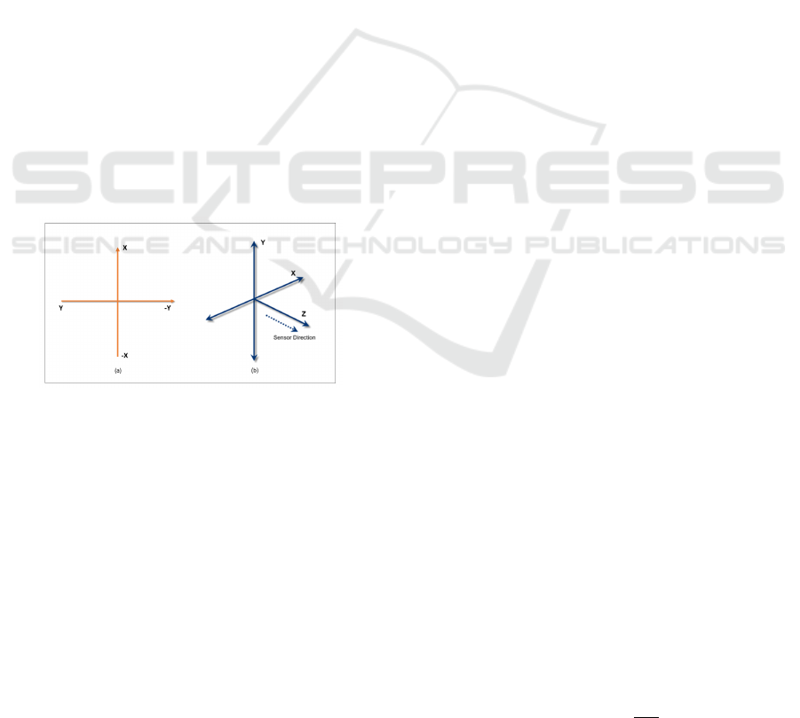
3.1 Local Map and Coordinates
Our system was developed taking as reference the lo-
cal map and the coordinate system of the Turtebot.
This local map is presented in the Fig. 1 (a). In the
map, x is the abscissas, the distance ’in front’ of the
robot, and y is the ordinate coordinate on the plane.
This coordinates are defined by the Turtebot on ini-
tialization, and are used as the standard reference for
the APF. The Turtebot orientation is retrieved by its
on-board compass sensor.
Figure 1: Local map coordinates scheme of the ’Turtlebot
2’ (a) and the coordinate system of the RGB-D kinect sensor
(b).
3.2 Repulsive Field and Force
At first step, the Kinect data is processed by the PCL
as a point cloud. In our algorithm, two filters are
applied to the input point cloud to reduce the area
and, consequently, the number of points. First, the
voxel grid reduces the number of points in the point
cloud, defining the minimal distance of 0.01 m be-
tween the points of our interest, which increases the
performance of the algorithm. Then, one passthough
is applied to each coordinate, defining a box, as the
focus of interest in the cloud. For our work, we con-
sider only this area of interest, where the Turtlebot is
capable to move. The specified dimensions must be
bigger than the size of the robot, in order to allow its
to detect close obstacles on the sides as well as hori-
zontal barriers, such as a table.
Then, having the resulting cloud P, we applied
the Euclidean Extract method of PCL to form clusters
(PCL, 2016a). This method divides the unorganized
cloud P into smaller parts (sub-clouds), that reduces
the processing time for P. This method consists of
four steps:
1. Create a Kd-tree representation for the input cloud
P (PCL, 2016b);
2. Set up an empty cluster C, and a queue of points
to be checked Q;
3. Then for every point p
i
∈ P, is done:
add p
i
to the current queue Q;
for every point p
i
∈ Q, search for the set P
k
i
of points neighbors of p
i
in a sphere with radius r
¡ d
(
th);
for every neighbor P
i
k ∈ P
i
k check if the
point has been already processed, if not, add it to
Q.
when all points p
i
∈ P have been processed,
we receive the clusters projected.
The repulsive field is extracted from the Kinect
data, that is clusters identified by the coordinates x,y,z
of the Kinect, which is different from that of the local
map. Fig. 1 (b) shows the kinect sensor coordinate
system.
To compute the repulsive field intensity, we calcu-
late the Manhattan distance, on the plane, between the
robot and each point in the identified clusters. So, for
the ith point in the cluster, the Manhattan distance is:
d
i
= |x
(k)
i
| + |z
(k)
i
| (1)
We adopt a linear potential in the form:
V
i
= λ{1 − d
i
/D
max
}, (2)
where D
max
is biggest Manhattan distance in the box
defined by the passthough filter, and λ is a constant.
To calculate the modulus of the force attributed to this
potential field, all we need to do is take the derivative:
|F
i
| = −λ/D
max
, (3)
which is a constant for all points in the cloud. The
direction, though, is the important information, for it
is responsible to orientate the robot away from the ob-
stacle. It can be defined by the angle:
θ
i
= arctan
x
(k)
i
z
(k)
i
!
, (4)
ICAART 2017 - 9th International Conference on Agents and Artificial Intelligence
310

which implies in the force:
F
( ˆx
(k)
)
i
= −sin(θ) × λ/D
max
(5)
F
(ˆz
(k)
)
i
= −cos(θ) × λ/D
max
(6)
Then, the resulting repulsive force is just the sum
of the forces by each point in the cluster:
F
( ˆx
(k)
)
rep
= λ /D
max
∑
i
sin(θ), (7)
F
(ˆz
(k)
)
rep
= λ /D
max
∑
i
cos(θ), (8)
with a modulus:
|F
rep
| =
q
(F
( ˆx)
rep
)
2
+ (F
(ˆz)
rep
)
2
(9)
It is important to notice that this force is repre-
sented in the coordinate system of the Kinect, which
is mounted in the robot, and thus can be both trans-
lated and rotated in relation to the local map coordi-
nate, at any moment. Considering that the robot is
rotated by an angle ϕ in relation to the local map co-
ordinate, the resulting repulsive force can be written
in the local coordinate as:
F
( ˆx)
rep
= sin(ϕ)λ /D
max
∑
i
sin(θ) +
+cos(ϕ)λ /D
max
∑
i
cos(θ), (10)
F
( ˆy)
rep
= −cos(ϕ)λ /D
max
∑
i
sin(θ) +
+sin(ϕ)λ /D
max
∑
i
cos(θ). (11)
3.3 Attraction and Resultant Force
The attractive potential is responsible to direct the
robot towards the target (destination), and is com-
puted using the euclidean distance calculated from the
encoders data. We consider that the target exerts an
attractive, gravitational like, force in the system, that
is:
|F
att
| =
Λ
p
(x
a
)
2
+ (y
a
)
2
, (12)
where Λ is an intensity related constant and (x
a
,y
a
)
are the ˆx and ˆy distances, respectively, of the robot
from the target, calculated on the local map coordi-
nate system.
The angle of the target direction is gave by:
φ = arctan
y
a
x
a
, (13)
which implies in the components:
F
( ˆx)
att
=
cos(φ)Λ
p
(x
a
)
2
+ (y
a
)
2
, (14)
F
( ˆy)
att
=
sin(φ)Λ
p
(x
a
)
2
+ (y
a
)
2
. (15)
Therefore, the resulting force is just the sum of the
attractive and repulsive forces:
F
( ˆx)
res
= F
( ˆx)
att
+ F
( ˆx)
rep
, (16)
F
( ˆy)
res
= F
( ˆy)
att
+ F
( ˆy)
rep
, (17)
Now, all we have to do is calculate the modulus
and direction of this force, which are respectively:
|F
res
| =
q
(F
( ˆx)
res
)
2
+ (F
( ˆy)
res
)
2
(18)
ψ = arctan
F
( ˆy)
res
F
( ˆx)
res
!
(19)
4 ROBOT BEHAVIOR
In accordance with (Alejo et al., 2015), to avoid the
collision among the robot and the obstacles found in
the environment, it is possible to use the following
two reactions: speed change and/or direction change.
The Turtlebot is controlled by defining its linear and
angular velocity, v and ω respectively. So, in order to
correctly apply the resultant force to the robot dynam-
ics, we must first rotate it to align its orientation with
the resultant force direction. For that, we consider
the angle difference, and divide it by the Turtlebot re-
freshing time ∆t, and take it to be the angular velocity
of the robot in that time interval:
ω =
ψ − ϕ
∆t
. (20)
Then, we take the force modulus to be the varia-
tion of the linear velocity, in the time interval ∆t, that
is:
∆v
∆t
= |F
res
|. (21)
With this setup, the robot is able to effectively
avoid obstacles, in an stable manner, as will be shown
in the next section.
5 EXPERIMENTS
The experiments was performed using a Turtlebot 2
platform which is 60 cm high and 48 cm wide (mea-
sured with the laptop attached). We dont transform
A 3D Anti-collision System based on Artificial Potential Field Method for a Mobile Robot
311
the point cloud to a depth map (2D) because it present
the information of the entire visual field, whereas we
want to work with a limited region in space. Also, it
is fundamental for our algorithm to have height infor-
mation. Instead, we use a voxelgrid and passthrough
filters to decrease the number of points and create a
focus window, then it is applied the KNN algorithm
to get the points of interesting and building a unique
cluster, finally it is generated the force on each point
according to distance of each point to the kinect sen-
sor.
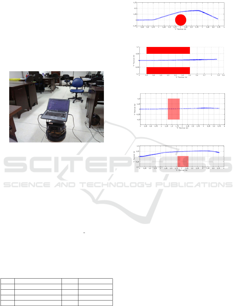
Figure 2: The ’Turtlebot 2’ avoiding the obstacle (chair) in
first challenge.
The voxel grid considered only points within at
least 1 cm of each other. The passthrough reduces
the area to 1.8m in each direction of ˆx, −0.1m to
2.5m in ˆy and 0.0m to 6.0m in ˆz, coordinates of the
Kinect. To build the Kd-tree, extracting clusters with
PCL method, the euclidean distance was defined as 2
cm, and the response time was high, with a measured
refresh rate of 5 Hz.
The four kind of challenges used as base to
prove the efficiency of our algorithm can be found
in the video ”Artificial Potential Field Algorithm” in
https://www.youtube.com/watch?v=gH pNfC8gP8&
feature=youtu.be. It shows the positive results
achieved using this new algorithm, and the table 1 list
the challenges surpassed by this method proposed in
this work.
Table 1: The four different challenges surpassed by our al-
gorithm using the mobile robot, Turtlebot.
Exp. Challenges Target Narrow passages
1 avoiding obstacle 4.0 m -
2 passing between barriers 3.5 m 70 cm (wide)
3 passing under the table 4.0 m 73 cm (high)
4 circumventing the table 4.0 m 40 cm (high)
After a battery of tests, the best parameters found
for these challenges, were:
• Λ = 2.7
Figure 3: The path made by the ’Turtlebot 2’ in the first
experiment.
Figure 4: The path made by the ’Turtlebot 2’ in the second
experiment.
Figure 5: The path made by the ’Turtlebot 2’ in the third
experiment.
Figure 6: The path result made by the ’Turtlebot 2’ during
one test of the fourth experiment.
• λ = 0.4
• D
max
= 1.5
• The linear speed: min = 0.0, max = 0.2
• The angular speed: min = 0.0, max = 0.2
The target, which offers an attractive force for
the Turtlebot, in the experiments 1, 3 and 4, was de-
fined as 4m forward, and for the experiment 2, the tar-
get was defined as 3.5m because of space restriction.
The distance from the target was updated over time,
through the encoders data of the robot (coupled at the
wheels) and its compass. These data enabled tracking
the Turtlebot, returning its pose (position and orienta-
tion).
The system performed very well at all challenges.
However, the system had some difficulty to find a way
to escape of an imminent collision when the obstacle
is very wide, as a table with 1.5 m wide and 1.2m high
(experiment 4). For this, it was necessary to reduce
the maximum linear speed of 0.2 to 0.1. That aided
the vision node to have enough time to build the Kd-
tree without problems.
With these parameters, the system was able to
ICAART 2017 - 9th International Conference on Agents and Artificial Intelligence
312

avoid collision with the obstacles, passing between
closely spaced obstacles, exhibiting no oscillations in
the presence of obstacles, no oscillations in narrow
passages and reaching its target with success.
6 CONCLUSIONS
As shown by the performed experiment, our proposed
modified potential field method was able to surpass
all proposed challenges. The robot was able to avoid
obstacles, find a passage between closely spaced ob-
stacles, pass beneath higher obstacles and avoid high
obstacles that did not allowed it to pass underneath,
all in a smooth and oscillation-free manner.
We understand there is ample space for improve-
ment of our technique, specially if it is to work on
highly dynamical environments, with moving obsta-
cles. In this regard we believe performance improve-
ments are needed.
REFERENCES
Alejo, D., Cobano, J., Heredia, G., and Ollero, A. (2015).
Collision-free trajectory planning based on maneuver
selection-particle swarm optimization. In Unmanned
Aircraft Systems (ICUAS), 2015 International Confer-
ence on, pages 72–81.
Anthony Cowley, William Marshall, B. C. and Taylor, C. J.
Depth space collision detection for motion planning.
Bentes, C. and Saotome, O. (2012). Dynamic swarm for-
mation with potential fields and a* path planning in 3d
environment. In Robotics Symposium and Latin Amer-
ican Robotics Symposium (SBR-LARS), 2012 Brazil-
ian, pages 74–78.
Borenstein, J. and Koren, Y. (1988). Obstacle avoidance
with ultrasonic sensors. Robotics and Automation,
IEEE Journal of, 4(2):213–218.
Chen, X. and Zhang, J. (2013). The three-dimension path
planning of uav based on improved artificial potential
field in dynamic environment. In Intelligent Human-
Machine Systems and Cybernetics (IHMSC), 2013 5th
International Conference on, volume 2, pages 144–
147.
Elfes, A. (1987). Sonar-based real-world mapping and nav-
igation. Robotics and Automation, IEEE Journal of,
3(3):249–265.
Fonnegra Tarazona, R., Rios Lopera, F., and Goez Sanchez,
G.-D. (2014). Anti-collision system for navigation
inside an uav using fuzzy controllers and range sen-
sors. In Image, Signal Processing and Artificial Vision
(STSIVA), 2014 XIX Symposium on, pages 1–5.
Hameed, I., la Cour-Harbo, A., and Osen, O. (2016). Side-
to-side 3d coverage path planning approach for agri-
cultural robots to minimize skip/overlap areas be-
tween swaths. Robotics and Autonomous Systems,
76:36 – 45.
Hwang, Y. and Ahuja, N. (1992). A potential field ap-
proach to path planning. Robotics and Automation,
IEEE Transactions on, 8(1):23–32.
Khuswendi, T., Hindersah, H., and Adiprawita, W. (2011).
Uav path planning using potential field and modified
receding horizon a* 3d algorithm. In Electrical Engi-
neering and Informatics (ICEEI), 2011 International
Conference on, pages 1–6.
Kong, L.-K., Sheng, J., and Teredesai, A. (2014). Basic
micro-aerial vehicles (mavs) obstacles avoidance us-
ing monocular computer vision. In Control Automa-
tion Robotics Vision (ICARCV), 2014 13th Interna-
tional Conference on, pages 1051–1056.
Liang, X., Wang, H., Li, D., and Liu, C. (2014). Three-
dimensional path planning for unmanned aerial vehi-
cles based on fluid flow. In Aerospace Conference,
2014 IEEE, pages 1–13.
Mac, T. T., Copot, C., Hernandez, A., and Keyser, R. D.
(2016). Improved potential field method for unknown
obstacle avoidance using uav in indoor environment.
In 2016 IEEE 14th International Symposium on Ap-
plied Machine Intelligence and Informatics (SAMI),
pages 345–350.
Nascimento, T. P., Conceicao, A. G. S., and Antonio P. Mor-
eira, k. . (2014). Multi-robot systems formation
control with obstacles avoidance. 19th IFAC World
Congress on International Federation of Automatic
Control IFAC 2014 24 August 2014 through 29 August
2014, 19:–.
PCL (2016a). Euclidean cluster extraction. Access date: 22
jun. 2016.
PCL (2016b). How to use a kdtree to search. Access date:
22 jun. 2016.
Santos, M., Santana, L., Brandao, A., and Sarcinelli-Filho,
M. (2015). Uav obstacle avoidance using rgb-d sys-
tem. In Unmanned Aircraft Systems (ICUAS), 2015
International Conference on, pages 312–319.
Scaramuzza, D. and Fraundorfer, F. (2011). Visual odom-
etry [tutorial]. Robotics Automation Magazine, IEEE,
18(4):80–92.
Souza, A. and Maia, R. (2013). Occupancy-elevation grid
mapping from stereo vision. In Robotics Symposium
and Competition (LARS/LARC), 2013 Latin Ameri-
can, pages 49–54.
Tan, F., Yang, J., Huang, J., Jia, T., Chen, W., and Wang, J.
(2010). A navigation system for family indoor mon-
itor mobile robot. In Intelligent Robots and Systems
(IROS), 2010 IEEE/RSJ International Conference on,
pages 5978–5983.
Zhu, L., Cheng, X., and Yuan, F.-G. (2016). A 3d colli-
sion avoidance strategy for {UAV} with physical con-
straints. Measurement, 77:40 – 49.
A 3D Anti-collision System based on Artificial Potential Field Method for a Mobile Robot
313
