
Optimization and Scheduling of Queueing Systems for Communication
Systems: OR Needs and Challenges
Attahiru Sule Alfa
1,2
and B. T. Maharaj
2
1
Department of Electrical and Computer Engineering, University of Manitoba, Winnipeg, MB, Canada
2
Department of Electrical, Electronic and Computer Engineering, University of Pretoria, Pretoria, South Africa
Keywords:
Optimization, Scheduling, Queueing, Congestion Control, Network Performance, Cognitive Radio Networks,
Wireless Sensor Networks, Internet of Things.
Abstract:
The modern communication system is growing at an alarming rate with fast growth of new technologies to
meet current and future demands. While the development of devices and technologies to improve and meet the
expected communication demands keeps growing, the tools for their effective and efficient implementations
seem to be lagging behind. On one hand there is a tremendous development and continued advancement of
techniques in Operations Research (OR). However it is surprising how the key tools for efficiently optimizing
the use of the modern technologies is lagging behind partly because there isn’t sufficient cooperation between
core OR researchers and communication researchers. In this position paper, using one specific example, we
identify the need to develop more efficient and effective OR tools for combined queueing and optimization
tools for modern communication systems. OR scientists tend to focus more on either the analysis of commu-
nication issues using queueing theory tools or the optimization of resource allocations but the combination of
the tools in research have not received as much attention. Our position is that this is one of major areas in the
OR field that would benefit communication systems. We briefly touch on other examples also.
1 INTRODUCTION
The demand for communication systems keeps grow-
ing on an ongoing basis. Communication industry
researchers are continuously working at coming up
with new technologies for meeting the demands. In
a recent ACG Research report (ACG, 2015) it was
pointed out that for an area of 1,200 square kilome-
ter metro area having approximately a population of
about 2.5 million people the bandwidth requirement
for backhaul at a cell site could be as high as 2.5
Gbps in the year 2018 and about 10 Gbps of Ether-
net links and 10 Gbps rings to meet the demand re-
quirements and support the expected growth. Part of
these growths in demand have to do with the shifts
in customers to data. In the past media and video
was less than 10% of the traffic and now it is almost
50% according to the recent Global telecommunica-
tions study: navigating the road to 2020 (EYReport,
2015). Bandwidth available is limited however efforts
are been made to squeeze more from what is avail-
able and also to release some inefficiently utilized ra-
dio frequencies for other uses. Hence telecommuni-
cation engineers do not only have to ensure that they
could provide the capacity for these demand growths
but make sure also that the capacity is efficiently well
managed.
In trying to provide efficient and effective com-
munication services for the future we need to harness
several key tools mostly OR based. Our position is
that this has not received the proper attention it de-
serves from the OR researchers and practitioners. The
aim of this paper is to try, with the aid of some ex-
amples, to identify the major role that OR researchers
can play in planning modern communication systems.
Historically queueing model by itself has been ex-
tensively used in analyzing the performance of com-
munication systems. In fact to the extent that when
people talk of performance analysis in communica-
tion systems they are most likely referring to queue-
ing model analysis of a communication system. Of-
ten the model is for a particular protocol. A protocol,
in simple terms, is the rule by which a system oper-
ates. When the protocol for a system changes, the
queueing system that represents it changes and hence
the system would need to be re-modelled in order to
obtain its performance. Keeping in mind that a com-
munication system designer may have a plethora of
430
Sule Alfa A. and Maharaj B.
Optimization and Scheduling of Queueing Systems for Communication Systems: OR Needs and Challenges.
DOI: 10.5220/0006235504300439
In Proceedings of the 6th International Conference on Operations Research and Enterprise Systems (ICORES 2017), pages 430-439
ISBN: 978-989-758-218-9
Copyright
c
2017 by SCITEPRESS – Science and Technology Publications, Lda. All rights reserved

possible protocol designs for a particular system, de-
ciding on the ”best” design becomes an exercise of
modelling and evaluating the system with each pro-
tocol and evaluating it. This could be a nightmare
of combinatorial problem. The ideal thing would be
to be able to develop a combined queueing and op-
timization model where the parameters of the queue-
ing system are to be decision variables in the opti-
mization problem and a performance measure of the
system is the objective function. This is straightfor-
ward enough. However when we look at the literature
on this subject the research on the topic lags behind
considerably in meeting the challenges of appropriate
mathematical modelling of the modern communica-
tions needs. That is why we have decided to further
bring this to the attention of OR researchers and ana-
lysts.
2 COGNITIVE RADIO
NETWORKS
Cognitive radio networks (CRN) is one of those tech-
nologies that is being pursued as a way to increase
capacity for communication. CRN emerged from the
observations of some researchers and the FCC (Fed-
eral Communications Commission) that some of the
licensed frequencies, especially the TV band, are un-
derutilized. As a result CRN is a network in which
when the primary user (who has license for a partic-
ular channel) is not using it a secondary user may try
and access it provided it does not interfere (beyond
a tolerable limit) with the primary user. For more de-
tails about this technology and associated background
see (Mitola and Maguire, 1999) and (Haykin, 2005).
In CRN a secondary user (SU) senses a channel
and may access it if it is not in use. We call this ac-
cess approach the overlay. However if the channel is
in use by the primary user (PU) the SU may still ac-
cess it if the SU can transmit at a power level that will
not interfere with the PU. This we call the underlay.
The methods for sensing the channels are well docu-
mented in the communication literature.
The question here is when a channel can be ac-
cessed by SUs how does the system decide on which
SU to access which the channel and for how long.
This becomes a major queueing and optimization
problem which is better addressed by using OR tools.
In the next section we show how OR tools can be con-
sidered as tools for this and the challenges involved.
In real life there are several channels involved in
communication systems. However to make it simple
for expositional purposes we consider a single chan-
nel model for CRN. Later we discuss how the multiple
Busy
Idle
Fig 1. Busy and Idle times (single channel)
Time
Figure 1: Busy and Idle times (single channel).
channel cases are studied.
Consider a single communication channel used by
one or several PUs. For simplicity let us assume that
the PUs arrive according to a Bernoulli process with
parameter λ
p
and the channel can process at geomet-
ric distribution with probability µ. Keep in mind that
the PUs required processing rate could be µ
p
< µ.
This system can be studied as the Geo/Geo/1 queue.
Even if the arrival and processing processes are not
simple we can still analyze the system using a sin-
gle server queueing model. We chose to work in dis-
crete time because modern communication systems
are digital. Further consider a case on one channel
licensed to a PU which is either busy or idle. We
can represent it as an alternating stochastic process
{busy, idle}. A simple example of that is an alter-
nating Markov renewal. For the sake of explaining
we consider the special case of Markov chain, with
two states {0, 1} where 0 represents busy and 1 rep-
resents idle. Let X
n
be the state at time n and define
P
i, j
= Pr
{
X
n+1
= j, X
n
= i
}
, ∀n then we can write the
transition matrix of this system as
P =
p
0,0
p
0,1
p
1,0
p
1,1
The following diagram (Fig. 1) is a schematic rep-
resentation of idle and busy periods of this channel.
If we now introduce an SU with arrival probability
λ
s
, this SU may try and access the channel using the
overlay or underlay schemes.
2.1 Overlay Scheme
In the overlay scheme, the SU will only access the
channel when it is idle and has to vacate it when the
PU returns to the channel, i.e. when it becomes busy
again. So in essence an SU sees this channel as a va-
cation queueing system in which the server (channel)
is on vacation when it is busy with the PU. The SU
can thus only be served during the queues idle period
(when the PU is not occupying it). This is a queueing
problem which can be analyzed using standard queue-
ing models. This problem is quite straightforward if
all we have is just one SU trying to access the channel.
The SU just waits for the time it detects the channel
to be idle and then access it. The point in time when
Optimization and Scheduling of Queueing Systems for Communication Systems: OR Needs and Challenges
431
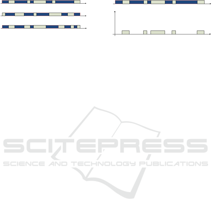
Time
Time
Time
Fig 2. Busy and Idle times (multiple channel)
Channel 1
Channel 2
Channel 3
Figure 2: Busy and Idle times (multiple channel).
the channel becomes idle is a point process and the
duration of the idle period is stochastic.
The question that arises then is when we have
more than one SU waiting to access the channel; how
do we allocate the channel to the SUs? What prior-
ity schemes do we use? This calls for an optimiza-
tion tool for scheduling the SUs. Keeping in mind
the stochastic nature of the idle and busy periods of
the channel a system scheduler has to implement an
efficient scheduling procedure. Now if we have mul-
tiple channels, which is more realistic, then we are
dealing with a system of superposition of several of
the channel Markov chains. For simplicity let us as-
sume that the channels are identical with the same
Markov chains with representation P, then the result-
ing Markov chain that represents all the K channels
has Markov chain with transition matrix P
K
written as
P
K
= P ⊗ P ⊗ · ·· ⊗ P,
where there are K Kronecker products of the matrix
P , i.e. P
K
=
N
K
j=1
P. A good diagrammatic example
of the busy and idle channel behaviours of this can be
demonstrated by the case of K = 3 in Fig. 2.
In this case we need to keep track of which queue
(channel) is idle and which one is busy at all times.
Selecting which channel to assign to which SU is a
challenging dynamic assignment problem; scheduling
when to let a particular SU access a channel is also
a challenging OR problem, especially if we assign a
group of channels to some SUs ((Jiao et al., 2011; Jiao
et al., 2012)).
Finally there are usually some SUs that have high
data transmission rate and often are willing to pay for
superior service. Such SUs require that more than one
channel are assigned to them ((Jiao et al., 2011; Jiao
et al., 2012)). How do we develop an optimization to
handle this type of problem? For example, consider
the case of three identical channels above. If we have
say three SUs, and one of them requires two chan-
nels while the third channel is shared by the other
two, how do we decide which two channels to as-
sign to this special SU? There are three possible ways,
all dependent on the stochastic process describing the
channels. One just has to imagine what happens when
we have N (N >> 1) channels and M (M >> 1) SUs
with the i
th
SU requiring m
i
channels. . Even for the
Capacity
Time
Time
Fig 3. Capacity (single channel)
Figure 3: Capacity (single channel).
case when
∑
M
i
m
i
≤ N it could still be a major combi-
natorial problem, combining queueing and optimiza-
tion.
These are some of the issues that arise in the CRN
technologies, and which we think can benefit tremen-
dously from the OR communities.
2.2 Underlay Scheme
Dealing with the underlay scheme is about the same
as the overlay scheme except that we now have to also
allocate a power level to an SU to ensure that it does
not interfere with a PU transmission. So the addi-
tional question here is what power level should we
assign to an SU and to which SU in order to maxi-
mize communication capacity?
In addition we may also be in a position to have
a hybrid scheme in which some SUs are placed on
overlay scheme, some on underlay scheme and some
on a combination of both. The question is how do
we determine which ones to assign what scheme and
how? This is an optimization problem which also has
impact of the network performance.
Let us first look at the case of one channel in
which an SU wants to consider underlay in addition
to overlay, i.e. a hybrid. For the one channel even
though we may know the busy and idle period, during
the idle period we know that an SU can transmit at its
full power (if possible), if it is the only one transmit-
ting. However if it wants to transmit also under the
underlay scheme the power level allowed may vary
depending on what is the level of power of the PU.
We present a schematic diagram of the situation under
full capacity below in Fig. 3, i.e. when the channel is
idle. For the case of underlay,he available capacity
cannot be higher than what is shown in Fig. 3.
If we now consider the case of three channels, su-
perimposed and then capturing the combined capacity
we may have a case like the one below in Fig. 4.
How to now assign the channels and power be-
comes a major queueing, assignment and scheduling
problem which is not as straightforward.
In what follows we introduce a small generic re-
source allocation problem and use that as the basis of
our discussions in comparing the papers in the liter-
ICORES 2017 - 6th International Conference on Operations Research and Enterprise Systems
432
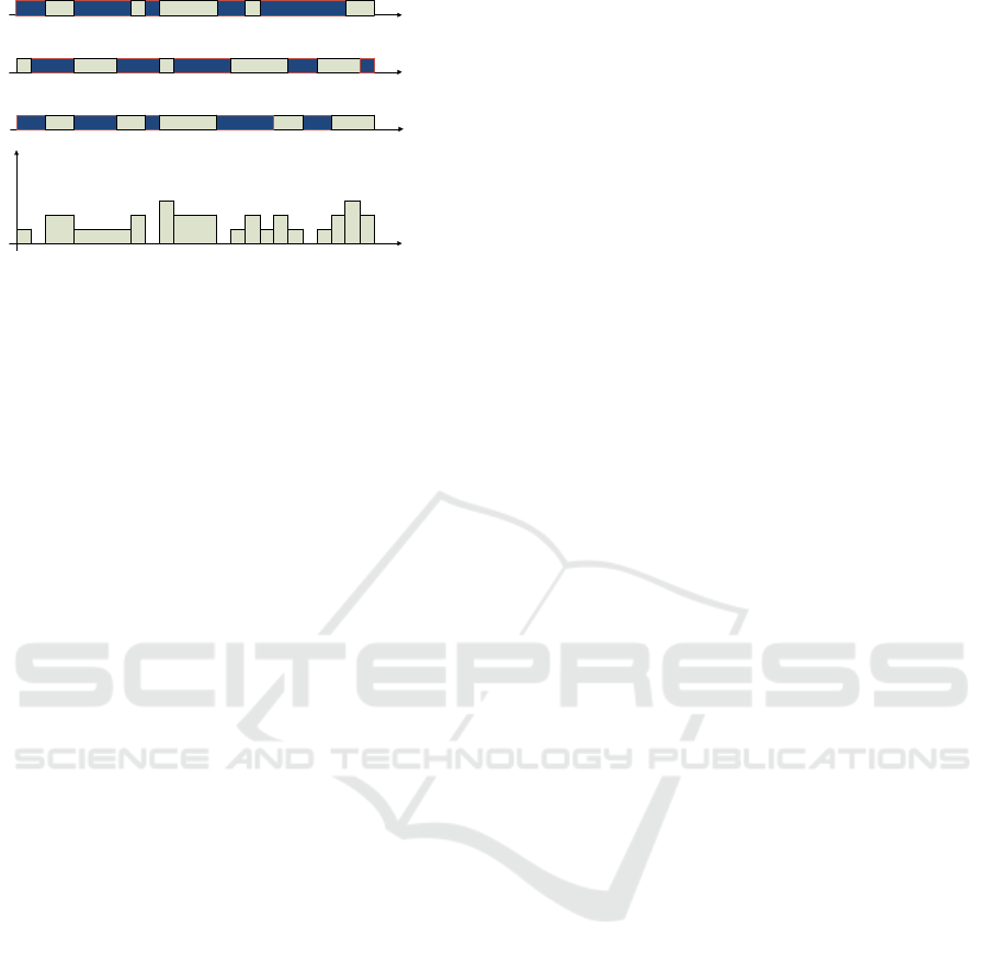
Time
Capacity
Time
Time
Time
Channel 1
Channel 2
Channel 3
Fig 4. Capacity (multiple channels)
Figure 4: Capacity (multiple channel).
ature. Consider a simple CRN problem in which we
have K PU channels. There are M SUs looking for ac-
cess to the PU channels. Each SU, s = 1, 2, ··· , M has
a maximum power source of P
s
max
. If SU s is allowed
to transmit on channel k with power level P
s
k
, then
its capacity, c
s
k
will be given as c
s
k
= log
1 + γ
s
k
P
s
k
,
where γ
s
k
is the noise level associated with SU s trans-
mitting on channel k. This is essentially a simplified
Shannon’s capacity formula or a formula derived from
it. Whether we are dealing with capacity, throughput
or data rate a version of this formula is what we use.
Let x
s
k
= 1 if channel k is assigned to SU, s and
zero, otherwise. Generally the throughput and data
rate resulting from this are directly proportional to
this capacity. So in essence the total capacity assigned
to this SU, s will be
z
s
=
K
∑
k=1
c
s
k
x
s
k
.
In RA problem our interest would be to maximize
the total weighted capacity for all the SUs, with the
weight w
s
assigned to SU s. Hence the objective func-
tion of this generic problem will be
max z =
M
∑
s=1
w
s
K
∑
k=1
c
s
k
x
s
k
. (1)
This is a non-linear function in P
s
k
and x
s
k
.
Next we consider the constraints. The first one
is that we want to ensure that at least one channel is
assigned to an SU, on the assumption that M ≤ K. So
we need the constraint
K
∑
k=1
x
s
k
≥ 1, ∀s = 1, 2, ··· , M, (2)
and also a constraint that ensures that we do not assign
more than a channel to more than one SU, i.e.
S
∑
s=1
x
s
k
≤ 1, ∀k = 1, 2, ··· , K. (3)
The next constraint is that we cannot allow the
total power generated by an SU to exceed its power
limit. So we need the constraint that
K
∑
k=1
P
s
k
≤ P
s
max
, ∀s = 1, 2, ·· · , M. (4)
A key requirement in CRN is that the SU should
not interfere with the PU, or at least the interference
should not exceed the maximum allowed level. This
can be easily captured by requiring that the power
reaching the PU should not exceed a particular value
P
power
. So the next constraint is
S
∑
s=1
K
∑
k=1
P
s
k
γ
s
k
≤ P
power.
(5)
with the variables allowed to assume any non-
negative values.
Given that SUs usually have a minimum require-
ment for QoS we assume that there is a constraint in
this regard also. For example, an SU, s, may require
a minimum of σ
s
of total capacity after combining a
number of sub-channels assigned, so this leads to the
constraint
K
∑
k=1
x
s
k
c
s
k
≥ σ
s
, ∀s = 1, 2, ·· · , M. (6)
Finally we have the two critical but common con-
straints, i.e. that of zero-one on x
s
k
and non-negativity
on P
s
k
, both written as
x
s
k
∈
{
0, 1
}
. (7)
P
s
k
≥ 0. (8)
In summary, Equations (1) to (8) form the re-
source allocation (RA) problem for this simple exam-
ple. As one can see, in its simplest form, the objec-
tive function in non-linear, and constraint (6) is non-
linear. Also one variable, x
s
k
is zero-one while P
s
k
is
a simple non-negative variable. So unless there is a
significantly different problem studied, non-linearity
and integer variables (zero-one) are unavoidable in
the formulations. That is why in general we have a
non-linear mixed integer programming problem for
RA. The issue now is how it has been handled in the
literature. A more detailed discussion of this can be
found in (Alfa et al., 2016).
It is however important to point out some aspects
of this formulation that could be further improved to
reflect an attempt to truly optimize the system as a
whole. We know that the resulting capacity available
to an SU, after the optimization, determines the de-
lay or latency of packet transmission. So we need to
incorporate additional constraints, based on queueing
Optimization and Scheduling of Queueing Systems for Communication Systems: OR Needs and Challenges
433

models, that limit the delay or add a delay cost com-
ponent to the objective function. These are usually not
incorporated in the RA models because of the com-
plexity it would introduce to the problem. This is one
major reason why it is important for the communica-
tion system researchers and OR analysts/researchers
need to collaborate on carrying out major complete
model analysis.
SUGGESTED IDEA FOR COLLABORATION:
Telecommunication researchers often resort to the
use of simple heuristics to quickly obtain solutions
to the type of optimization problems discussed
above. The heuristics are usually not rigorously
studied before implementation. For example,
exploring and understanding how “good” the
solutions are is very important especially now that
there is a need to “squeeze” as much as possible
from the network. Solutions that are not proven
to be efficient, for example if the gap between
the solution and the bound is large, could be
misleading. This is where it is very important for
the telecommunication researchers to collaborate
more with OR analysts whose interests, capacity
and experience are in these aspects. The OR
analysts on their own, would probably have more
interests in the mathematical analysis of the
system and looking for bounds. In the process
may assume away some important aspects of the
problem which a telecommunication researcher
knows is very important for the problem. That is
why the two groups need to collaborate and work
together in coming up with better solutions. The
combined collaborative effort of the two groups
would lead to much better solution.
3 WIRELESS SENSOR
NETWORKS AND THE
INTERNET OF THINGS
The Internet of things (IoT), which is probably more
correctly be termed the Internet for Things (IfT) as
suggested by Kevin Ashton, the originator of the term
IoT (Peter Day’s World of Business, 2016 (BBC,
2016)), is seen as one of the technologies that would
drive our daily activities and hence very important.
To quote the Wikipedia,“IoT is the internet working
of physical devices, vehicle, building and other items
embedded with electronics, software, sensors, actu-
ators, and networking connectivity that enable these
objects to collect and exchange data”. It is immedi-
ately clear that one of the technologies that would en-
able the IoT is wireless sensor networks, among many
other technologies. A wireless sensor network (WSN)
is a self-organizing network that consists of a number
of sensor nodes deployed in a certain area. The sen-
sor nodes basically sense and acquire data from the
environment, process data for storage, as well as a
communicate (transmit) the data to a sink node. It
is the communicated data that the IoT system uses
to actuate activities in response thereby generating
device-to-device activities. With the new 5G tech-
nology in discussion it is believed that the IoT will
drive most of actions and activities from smart cities
to smart grid, to smart health, environmental monitor-
ing, infrastructure management, manufacturing, en-
ergy management, city management, home and build-
ing automation, transportation, etc. So first we con-
sider the role of OR in sensor networks modelling and
analysis.
3.1 Wireless Sensor Networks
There are a number of different applications of sen-
sor networks in areas such as environmental moni-
toring, industrial control, disaster recovery, and bat-
tlefield surveillance. The major constraint in large
scale deployment of WSNs is the limited capacity of
processing, storage and energy of the wireless sensor
nodes. It is important that the buffer capacity is suf-
ficient to avoid data loss, that the processing capacity
is high enough to obtain very good latency, especially
for time sensitive data for the Internet of Things, and
most important is that processing is limited to times
when the system can be utilised efficiently, i.e. en-
ergy is conserved through the sleep/awake manage-
ment of the sensors. In order to effectively carry out
the design of many aspects of sensor networks, a very
good queueing analysis is important. Queueing the-
ory plays a major role than has been emphasized in
the literature.
WSN is a collection of several nodes of sensors
of all types connected via wireless channels of differ-
ent capacities with varying channel conditions. The
sensor nodes are usually of different capacities and
different functionalities. Some of them collect, pro-
cess and transmit data, and others only carry out a
few of the functions. Let us denote by N a set of sen-
sor nodes where N =
N
and N =
{
N
1
, N
2
, ···N
N
}
.
Let A be the set of channels connecting pairs of sen-
sor nodes. For example, let A
i, j
be a connection be-
tween sensor nodes N
i
and N
j
, then A is the set of
all those channels. Let C
i, j
be the capacity associ-
ated with channel A
i, j
, and K
i
as the buffer capacity
and P
i
as the processing capacity associated with sen-
sor node i. We can therefore say that a WSN can be
ICORES 2017 - 6th International Conference on Operations Research and Enterprise Systems
434

5
11
10
7 15
9
12
N
13
6
8
3
14
2
1
Sensor node
Fig. 5 Sensor node distribution
Sink node
Figure 5: Sensor node distribution.
described by a network G =
N , A
with attributes
(K
i
, P
i
), (C
i, j
), i ∈ N , (i, j) ∈ A
. See Fig. 5 as an
example.
1) Queueing Aspects of WSN: The first thing one
notices about WSN is that it is like a network of
queues with each sensor node representing a queue-
ing node. Since data arrival is usually not necessarily
Poisson type, and more often kind of correlated, sim-
ple single node queues or even simple queueing net-
work models such as the Jackson networks are not ap-
propriate for modelling the WSN. In addition, given
that we need to include sleep/awake mode schedul-
ing the model then becomes more complicated. This
calls for more sophisticated and more representative
queueing models, the types that queueing theoreti-
cians do not seem to have focused on yet. Consider-
ing queueing models that assume non-renewal types
of arrivals with bursty instances is more appropriate.
However then including such processes in a queueing
network, which is beyond the Jackson’s model, is a
challenge which queueing theorists need to tackle.
2) Power Management of WSN: Due to the fact
that most sensor nodes are battery operated, i.e. have
limited available power source, it is important to ef-
ficiently manage them effectively for a long lasting
network life. Usually a sleep/awake mode is im-
plemented to achieve this goal; a very good vaca-
tion queueing model in which the scheduling of the
sleep/awake mode is well controlled. This involves
a combined queueing model with optimization tech-
niques. Queueing theory can prove to be an effective
tool to analyze and design efficient power allocation
schemes to increase the power efficiency of WSNs
(see (Kabiri et al., 2014)). Sleep/awake models are
based on special kinds of vacation models. When
the sensor goes to the sleep mode, that means it is
switched off and cannot process data. This is es-
sentially a vacation model. Data arrivals accumulate
at the buffer. The node wakes up depending on the
time which is based on a policy of how many pack-
ets are waiting (N), how long they have been wait-
ing (T) and the total amount of Kilo-bytes of data
(D). These models are classified as N-policy, T-policy
or D-policy models. Recently there have been com-
bined versions of these models, such as the NT-policy,
and there are research activities going on regarding
developing ND, and NDT-policies. Sleep/wake-up
schemes essentially makes use of duty cycle schemes
which are used to wake a node up from an idle state
to the busy state by turning on the radio server. This
plays an important role in the level of power sav-
ings in the context of MAC protocols. The authors in
(Kabiri et al., 2014) derived an analytical model utilis-
ing a M/G/1 queue to model the sensor node; and by
altering the queue parameters, different sleep/wake-
up strategies were analysed. Some IEEE 802.11 MAC
protocols like the sensor MAC, sparse topology and
energy management, or the Berkeley MAC utilize a
queued wake-up where a threshold value is used to
control the average time of switching on a node and
the latency for buffered data packets. Determining the
optimal value of the packet queue length of a node af-
ter which the node is switched on for transmission, is
referred to as the N-policy. For more information see
(Jiang et al., 2012).
Let d
i
be the sum of the delays to data processing
at node N
i
and transmission from that node, and if
data is generated at node N
i
at the rate of λ
i
, then we
have
d
i
= d (λ
i
, P
i
, K
i
, T
i
), ∀i, (9)
and ω
i
th power consumption at that node, given as
ω
i
= ω(λ
i
, P
i
, K
i
, T
i
), ∀i. (10)
Given the appropriate parameters of the system we
can obtain the performance measures, whether we use
single node queueing models or queueing network
models.
3) Routing Aspects of WSN: Each sensor node
needs to send its data (processed or unprocessed) to
a sink node where decisions are taken for the whole
system, especially for the IoT to be implementable.
Apart from the usual link costs associated with net-
works in computing optimal routing paths for WSN
we also need to know the energy level at each node.
This aspect has to be incorporated in the routing algo-
rithm keeping in mind that there is a need to preserve
energy at nodes with low level of it. Hence routing
here considers costs of links and nodes. One other
tool that has been incorporated in routing for WSN
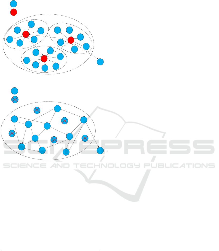
is selection of cluster head node which is responsible
for aggregating data from a group of nodes and then
transmitting to the sink node (see Fig.6). This routing
aspect for WSN is unique and has not received enough
attention from the OR researchers. As the 5G technol-
ogy is rolled out and the IoT developed to work using
Optimization and Scheduling of Queueing Systems for Communication Systems: OR Needs and Challenges
435
1
6
*
2 4
5
3
7
12
9
11
13
10
8
14 17
18
15
N
16
*
*
Sensor node
Fig. 6 Sensor node distribution with cluster heads
*
Cluster head
Sink node
Figure 6: SSensor node distribution with cluster heads.
5
11
10
7 15
9
12
N
13
6
8
3
14
2
1
Fig. 7 Sensor nodes in a depleting scenario
Sensor node
Dead node
Sink node
Figure 7: Sensor nodes in a depleting scenario.
that technology we want to maximize the technology
to ensure high effectiveness and efficiency. This calls
for the use of very effective and well researched OR
tools.
4) Reliability of WSN: The reliability of the WSN
is key to its effectiveness. It is important that if a sen-
sor node is not in operation due to low power or faulty
equipment, that data for the area can still be transmit-
ted. So we need very good reliability model that as-
sesses the impact of dead nodes as shown in Fig. 7.
SUGGESTED IDEA FOR COLLABORATION:
It is important that appropriate queueing models
are developed for WSN in order to obtain more
accurate estimate of delays at the nodes for the
purpose of providing efficient performance. Over-
simplified and inappropriate queueing models
lead to gross overestimation or underestimation
of performance measures leading to poor power
management and inefficient routing. It is very
common for telecommunication researchers to
assume Poisson arrivals, when often the arrival
process is far from that; and also ignoring corre-
lations in the arrival process is very common in all
the examples discussed in the last few sections. On
the other hand, OR analysts tend to be very rig-
orous by developing general models that are more
appropriate sometimes for unrealistic problems.
Combining the rigour of OR analysts with the re-
alistic view of the problems by telecommunication
researchers would lead to a very appropriate and
effective models. A good collaboration between
the two professions where more realistic models
are developed jointly and the effect of ignoring
some aspects of the systems are well understood
and accounted for would be the direction to go.
3.2 Sensor Node Placements
The placement of sensor nodes in a WSN is another
major factor in the reliability of WSN and its lifetime.
First in order for the WSN to be able to cover all areas
of interest the selection of the node placements have
to be selected strategically. For example, in (Cardei et
al., 2005) the optimization problem is to maximize the
number of set covers by selecting the optimal sensing
range for each sensor in each set cover while ensuring
each target is monitored by at least one sensor. This
problem is referred to as the Adjustable Range Set
Cover (AR-SC) problem and is initially formulated as
the following integer linear program: Consider N sen-
sor nodes s
1
, . . ., s
N
and M targets t
1
,t
2
, . . ., t
M
. Let the
sensor have P sensing ranges r
1
, r
2
, . . ., r
P
with corre-
sponding energy consumption e
1
, e
2
, . . ., e
P
. If E is
the initial sensor energy, and a
ip j
, a binary coefficient
which is 1 if sensor s
i
with radius r
p
covers the target
t
j
. Further let K be an upper bound for the number
of set covers. Then we have the following decision
variables:
Decision Variables:
c
k
, boolean variable for k = 1 . . . K, 1 if this subset is
a set cover
x
ikp
, boolean variable for i = 1 . . . N, k = 1. . . K, p =
1. . . P, 1 if sensor i with range r
p
is in cover k
The problem can now be set up as an integer linear
program (ILP) as
ILP:
maximize
K
∑
i=k
c
k
, (11)
s.t.
K
∑
k=1
P
∑
p=1
x
ikp
e
p
!
≤ E ∀i = 1 . . . N, (12)
ICORES 2017 - 6th International Conference on Operations Research and Enterprise Systems
436

P
∑
p=1
x
ikp
≤ c
k
∀i = 1 . . . N, k = 1 . . . K, (13)
N
∑
i=1
P
∑
p=1
x
ikp
∗ a
ip j
!
≥ c
k
∀k = 1 . . . K, j = 1 . . . M,
(14)
x
ikp
, c
k
∈
{
0, 1
}
. (15)
In (Cardei et al., 2005) the integer constraint is re-
laxed to create a linear programming problem which
is then used for the proposed LP based heuristic.
The LP based heuristic uses the values for each vari-
able obtained from solving the LP. The variables with
nonzero values from each cover set are added to the
new set in non-increasing order until all of the targets
are covered. This was improved further by the au-
thors in (Beynon and Alfa, 2015). If a sensor does not
have sufficient energy for the suggested power level
or does not cover any new targets it is not added to
the set. If no more nonzero variables are left for the
current cover and one or more targets remain uncov-
ered then the set is not a cover set. After the maximum
number of cover sets have been attempted to be made
the solution is the set of all valid cover sets.
SUGGESTED IDEA FOR COLLABORATION:
One may argue that this type of problem has been
well studied for years in OR as a class of problem
in the family of maximum covering location
problem. Yet telecommunication researchers still
have unanswered questions about coming up with
very good solutions for the maximum network
lifetime in wireless sensor networks. Perhaps this
is due to some subtleties in the later problem that
are probably ignored in the classical OR versions
of the problem. In our opinion this calls for more
close collaborations between the two groups of
researchers to understand the problem better and
its associated issues.
3.3 IoT
The IoT is essentially driven by the automatic or
“semi-automatic” control system. Data is sent from
some form of sensors, e.g. WSN, and based on the
data an action is taken as seen appropriate. For exam-
ple, a sensor network that is monitoring the temper-
ature at a building keeps gathering data and at each
point may notice that the temperature is too high and
thereby automatically control the system and lowers
the temperature. This is one of the most elemen-
tary ones. Another simple example could be a case
where as soon as a shopper in a grocery store is no-
ticed by a sensor network in the store a message is
sent to the shopper’s home refrigerator sensors which
then sends a message to the shopper’s mobile phone
to let him/her know they need more milk at home.
The communication here is what is called device-to-
device. However more important here is the need for
a process that determines that the milk has reached
low level or expired date etc and request the shopper
to purchase some. This is close to an inventory model
that is automated. The key difference is that there is
a time factor involved. The shopper has to be able to
get the message, from its mobile phone, when they
are still in the store otherwise it is not very helpful.
Hence latency is also a factor.
SUGGESTED IDEA FOR COLLABORATION:
This class of problem is more in the control
domain and requires a good collaboration be-
tween both OR analysts and telecommunication
researchers. It is still an evolving problem which
can benefit early from the collaborations.
In the next section we give a brief example of an-
other type of OR challenges for the future communi-
cation systems.
4 CONNECTING OPTIMIZATION
OF CRN AND QUEUEING OF
WSN
Currently WSN is operated on what is called the un-
licensed channels. These channels are getting con-
gested and it is being proposed that the licensed chan-
nels, which belong to PUs be used for transmitting
data in WSN. The sensor nodes are like queueing
nodes. Data is stored in the buffer and then transmit-
ted when possible. The transmission will be carried
out on licensed channels.
So here is the situation. Considering the PU chan-
nels, the SU, in this case the sensor node(s) will be
assigned a capacity c
s
k
on channel k from the opti-
mization model for CRN in Section III. However, be-
cause the assigned capacity and the number of allo-
cated channels are used by the SU to transmit the date
the latency depends on this which should actually be
incorporated as part of the optimization scheme in the
CRN problem. How to capture this feedback is a ma-
jor challenge. Here we present a possible example
method for dealing with it.
Let M be the number of sensor nodes in the WSN,
by trying to combine the two aspects then our Eq(1)
Optimization and Scheduling of Queueing Systems for Communication Systems: OR Needs and Challenges
437

in Section III will be
max z =
M
∑
s=1
"
ω
s
K
∑
k=1
c
s
k
x
s
k
− f (d
s
) − g(ω
s
)
#
, (16)
where f (d
s
) is the cost of delay at sensor node s and
g(ω
s
) is the cost of power consumption at node s.
We will also have Eq(9) and Eq(10) as additional
constraints for the optimization problem, in addition
to stability sets of equations.
SUGGESTED IDEA FOR COLLABORATION:
This will be a new and a bit more complex class of
problems. If we decide to include the placement
problem with this then the whole model becomes
very challenging. The question of how to manage
the problem should be of interest to OR analysts
who traditionally have the expertise to handle
them.
We suggest more close collaborations between OR
analysts and Communication network researchers.
5 CONCLUSIONS & THE
POSITION
We start by discussing the first example of cognitive
radio networks. Given the information about channel
capacity, which is usually stochastic, for SUs there are
several research results for allocating that resource to
the SUs using optimization tools. However, the allo-
cations provide the service capacity to the users and
hence a very good queueing model is needed to ob-
tain the performance analysis, which itself will now
feed back into the optimization tools. Hence what we
need is a combined queueing and optimization model
in order to efficiently model these systems.
Next we consider the wireless sensor networks,
we see that the optimal placement of the sensor nodes
determine network life, its reliability and routing
which affects latency. The placements, routing and
sleep/awake mode determines the queueing delays at
the nodes which need to be included in the optimiza-
tion component of the placements, etc. Hence for the
WSN, combined optimization and queueing models
are essential in order to have a well design WSN.
Finally, keeping in mind that an effective opera-
tion of IoT depends on accurately gathering informa-
tion and passing it to the right destination within a
very short time it is imperative that a combination of
optimization and queueing models are needed for the
planning.
In summary OR analysts and communication
modelling researchers need to try and work very
closely together in order to come up with efficient
tools for analyzing modern day communication sys-
tems. That is the position that we are taking in this
paper.
ACKNOWLEDGEMENT
The authors would like to thank the Advanced Sensor
Networks (ASN) South African Research Chairs Ini-
tiative (SARChI) for their financial support in making
this work possible. Thanks to Babatunde Awoyemi
for assisting with drawing the diagrams and to Dr.
Haitham AbuGhazaleh for assisting in recovering the
Latex file.
REFERENCES
Mitola, J. and Maguire, Jr., G. Q.(1999), Cognitive radio:
Making software radio more personal, IEEE Pers.
Communications, vol. 6, No. 4, Aug. 1999, 13-18.
Haykin, S. (2005), Cognitive radio: Brain-empowered
wireless communications, IEEE Journal of Selected
Areas of Communications, vol. 23, No. 2, Feb. 2005.
Jiao, L. Li, F.Y. and Pla, V. (2012), Modelling and per-
formance analysis of channel assembling in multi-
channel cognitive radio networks with spectrum adap-
tation, IEEE Trans. Vehicular Technology, 61 (6),
2686-2697.
Jiao, L. Li, F.Y. and Pla, V. (2011), Dynamic channel ag-
gregation strategies in cognitive radio networks with
spectrum adaptation, IEEE Globecom 2011, 1-6.
Alfa, A. S., Maharaj, B. T., Lall, S., and Pal, S. (2016),
Mixed-Integer programming based techniques for re-
source allocation in underlay cognitive radio net-
works: A survey, Journal of Communications and
Networks, vol. 18, No. 5, October 2016, 744-761.
Peter Day’s World of Business, BBC World Service, OC-
TOBER 4, 2016.
Beynon, V. and Alfa, A. S. (2015), An improved algo-
rithm for finding the maximum number of set covers
for wireless sensor networks, Africon, 2015.
Cardei, M., Wu, J., Lu, M. and Pervaiz, M. O. (2005), Max-
imum network lifetime in wireless sensor networks
with adjustable sensing ranges, IEEE International
Conference on Wireless and Mobile Computing, Net-
working and Communications, WiMob 2005 vol. 3,
pp. 438-445, 2005.
Kabiri, C., Zepernick, H. and Tran, H. (2014), On
Power Consumption of Wireless Sensor Nodes with
Min(N,T) Policy in Spectrum Sharing Systems, Pro-
ceedings IEEE Vehicular Technology Conference,
Spring 2014, 1-5.
ICORES 2017 - 6th International Conference on Operations Research and Enterprise Systems
438

Jiang, F., Huang, D., Yang, C. and Leu. F. (2012) Lifetime
elongation for wireless sensor network using queue-
based approaches, The Journal of Supercomputing,
vol. 59, no. 3, 1312-1335.
Forecasting of Mobile Broadband Bandwidth Require-
ments, ACG Research 2015, www.acgcc.com.
Global telecommunications study: navigating the road to
2020, 2015 report EY Building a better working
World.
Optimization and Scheduling of Queueing Systems for Communication Systems: OR Needs and Challenges
439
