
Deadlock Prevention in Rendezvous Generation for On-demand
Inter-robot Resource Delivery
Yin Chen, Xinjun Mao and Fu Hou
College of Computer, National University of Defense Technology, Changsha, Hunan, China
Keywords:
Deadlock, Rendezvous, Resource, Multi-robot System.
Abstract:
In this paper, we consider a multi-robot system (MRS) which executes task points associated with 2-D loca-
tions. Each task point demands certain physical resources for its execution. A robot can fetch these resources
either from fixed stations, or by conducting rendezvouses with other robots who happen to possess these
resources, provided that the latter option can be more beneficial in terms of cost or resource availability. How-
ever, applying rendezvouses may cause deadlock among robots, through (1) the tangling among rendezvouses,
or (2) sabotaging the resource consistency of the schedule of a robot which is originally holding the resources.
We analyse these problems and introduce a series of deadlock prevention rules that are embedded into an
A*-based rendezvous planning algorithm, so that both type of deadlocks can be avoided in the rendezvouses.
1 INTRODUCTION
Multi-robot systems (MRS) are applied in many do-
mains where their task execution requires retrieving
physical resources from the environment. The re-
quired resources may not be available in the vicinity
of a robot or may be held by other robots, making it a
desirable choice for a robot in urgent need of a partic-
ular set of resources to rendezvous with other robots
and fetch the resources from these robots, rather than
travel to the fixed resource stations which are either
far from the robot or depleted. Assume each robot
possesses a sequence of task points, each demanding
a specific set of resources, which can be fetched from
stations or via rendezvous with other robots. However
rendezvouses for resource delivery may cause two
types of inter-robot deadlocks which may block task
execution: (1) Rendezvous tangling, i.e., the ren-
dezvouses form a loop waiting for each other to com-
plete, blocking the execution forever. (2) Demand
looping, i.e., when all robots are self-interested, they
may be unable to achieve a globally feasible ren-
dezvous plan that satisfy each robot’s own demands
without jeopardising others’ demands.
In this paper we present deadlock prevention
mechanisms for the two types of deadlocks respec-
tively. The first type is tackled by constraining the
insertion index of each rendezvous so as to prevent
tangling. The second type is tackled by coordinating
the rendezvous planning on different robots so that
each rendezvous respects the demands of entire MRS
rather than only individual robots. We then present a
centralised A*-based algorithm (which will be trans-
formed into a distributed version in the future) that
searches for the best rendezvous insertion sequence
for satisfying the resource demands of entire MRS,
while respecting all the deadlock prevention rules.
2 RELATED WORK
Our work deals with the resource demands of sched-
ules of a MRS by dynamically generating ren-
dezvouses for fetching resources. In robotics litera-
ture, our work is similar in some way to the multi-
robot recharging problem, in which the robots (espe-
cially UAVs) rendezvous with ground-based charging
robots in order to charge their batteries. (Keshmiri,
2011) presents an opportunistic control approach to
address the multi-robot multi-rendezvous recharg-
ing problem, which combines centralised and dis-
tributed decision-making. (Neil Mathew, 2013) and
(Neil Mathew, 2015) present a method for multi-robot
recharging problem by modelling the rendezvous
planning problem into an integer linear program and
transform it into a travelling salesperson problem.
Despite their similarity: (1) our work considers het-
erogeneous demands by different task points for phys-
ical resources, and the types of resource are not lim-
ited to energy; (2) in stead of absolutely differenti-
670
Chen Y., Mao X. and Hou F.
Deadlock Prevention in Rendezvous Generation for On-demand Inter-robot Resource Delivery.
DOI: 10.5220/0006225806700675
In Proceedings of the 9th International Conference on Agents and Artificial Intelligence (ICAART 2017), pages 670-675
ISBN: 978-989-758-220-2
Copyright
c
2017 by SCITEPRESS – Science and Technology Publications, Lda. All rights reserved

ating between resource provider and consumer, we
make it possible for each robot to take any of both
roles according to the demands, so that the system can
more flexibly react to environment changes; (3) the
deadlock problem is raised because of the interdepen-
dency among different task points in the schedules,
which is largely omitted in the traditional recharging
problem. For the resource-caused deadlock problem,
(Han Lei, 2014) presents a Petri-Net-based multi-
robot scheduling approach for flexible manufacturing
system, which embeds deadlock control policies into
heuristic (e.g., genetic) search algorithm. Our work
is partially inspired by their idea of embedding dead-
lock prevention mechanisms into search algorithm.
In comparison, our work assumes dynamic environ-
ment and unforeseeable requirement resources, which
make our work potentially more applicable to a dy-
namic environment rather than a relatively fixed in-
dustrial environment.
3 PROBLEM FORMATION
3.1 Preliminaries
Task Point. Each task point π is a unit of task
execution on each robot, and is written as a tuple
hκ, l, R
, R
−
, R
+
i, where (1) κ is the action to be per-
formed by the robot to which the task point π is as-
signed; (2) l ∈ R
2
is the 2-D location at which the π
is to be executed; (3) R
is the set of resources re-
quired by π for its successful execution; (4) R
−
⊆ R
is the set of resources consumed by π; (5) R
+
is the
set of resources generated by π, provided that κ is a
resource-fetching action.
Schedule. Task points are organised into schedules
in order to be executed on robots. Each robot pos-
sesses a schedule σ which is defined as a sequence of
task points π
1
, ..., π
n
, where |σ| = n is the length of
the schedule. For each i = 1, ..., |σ|, σ(i) = π
i
is the
i
th
task point of the σ, and σ(0) is a presumed (but not
really existing) task point which marks the very be-
ginning of the schedule. The index of π is ι
σ
(π). For
each task point π ∈ σ, we make the following defini-
tions: (1) the set of task points preceding π is Π
(π) =
{π
0
∈ σ : ι
σ
(π
0
) < ι
σ
(π)}; (2) the set of task points
succeeding π is Π
(π) = {π
0
∈ σ : ι
σ
(π
0
) > ι
σ
(π)}.
Resource. Each resource r is defined as a tuple
hy, mi, where (1) y is the type of r; (2) m is the amount
of resource of type y shown by r. A set of resources
R can thus be defined as {r = hy, mi : y ∈ Y, m ∈ R}.
Operations of Resources. In this work, we assume
the resources are linear, and define their operations:
(1) hy, m
1
i + hy, m
2
i = hy, m
1
+ m
2
i; (2) hy, m
1
i −
hy, m
2
i = hy, m
1
− m
2
i; (3) k · hy, mi = hy, k · mi.
Operations of Sets of Resources. We define the
type set Y (R) = {y ∈ Y : ∃m ∈ R
+
: hy, mi ∈ R}. We
further define the operations (union, intersect, and mi-
nus) on set of resources: (1) R
1
˜
∪ R
2
= ς(R
1
∪ R
2
);
(2) R
1
˜
∩ R
2
= ς(R
1
∩ R
2
); (3) R
1
˜
\ R
2
= ς(R
1
∪ −R
2
),
where −R = {−r : r ∈ R}. The function ς is defined
as ς(R) = {r
0
∈
S
y∈Y (R)
{hy,
∑
r∈R,r.y=y
r.mi} : r
0
.m > 0},
which means that the resources with the same type
(r.y = y) will be combined into one, and all the re-
sources whose amount is below zero will be removed.
Required and Provided Resources. For each
schedule σ, and task point π ∈ σ, we can define:
(1) R
(π) is the set of resources required by π,
which is defined by R
(π) = π.R
; (2) R
(π) is the
set of resources provided by σ after executing π,
which is recursively defined by R
(σ(i)) = (R
(σ(i −
1))
˜
∪ π.R
+
)
˜
\ π.R
−
.
Resource Holder. This concept is introduced to
uniformly analyse the change of the resource config-
uration of the entire system (including both the MRS
and its environment). Each resource holder h is a tu-
ple hl, R, σi, where (1) l is the location of h; (2) R is
the set of resources currently possessed by h; (3) σ is
the sequence of task points which are not yet executed
and which will take effects on either the location l or
the set of resources R after being executed. A holder
h can be either a robot or a station. If h is a station,
then its σ field is simply a representation of those re-
sources scheduled to be given out to robots. If h is
a robot, then its σ field shows the sequence of task
points to be actually executed by the robot.
Rendezvous. Each rendezvous υ represents multi-
ple robots meeting at a common time and location,
and is defined as a tuple hl, Π, H, pi, where (1) l is
the location of the rendezvous; (2) Π is the set of task
points attending υ; (3) H is the set of resource hold-
ers attending υ; (4) p is a function which corresponds
each h ∈ H to π ∈ Π, so that p(h) = π shows that h
attending υ through executing π.
Resource-delivering Rendezvous. In this work, all
rendezvouses are used for delivering resources, and
therefore should contain only two task points: (1)
Deadlock Prevention in Rendezvous Generation for On-demand Inter-robot Resource Delivery
671
π
snd
for sending a set of resources R, which is exe-
cuted by the resource provider; (2) π
rcv
for receiving
a set of resources R, which is executed by the robot
demanding the resources. Thus for each resource-
delivering rendezvous υ, there exists π
snd
, π
rcv
, and
R, so that: υ.Π = {π
snd
, π
rcv
}, υ.H = {h
snd
, h
rcv
}, and
p = {hh
snd
, π
snd
i, hh
rcv
, π
rcv
i}.
3.2 Rendezvous Tangling
3
s
2
s
1
s
3
s
2
s
1
s
3
s
2
s
1
s
1 1
2 2
3 3
4 4
1
1
2 2
3
3
4 4
1 1
2 2
3
3
4 4
(a) Not tangled
(b) Two rendezvouses tangled
with each other directly
(c) Three rendezvouses tangled
with each other indirectly
1
u
2
u
3
u
4
u
4
u
4
u
1
u
2
u
1
u
3
u
2
u
3
u
The schedule of a robot
Task points of a rendezvous
A rendezvous
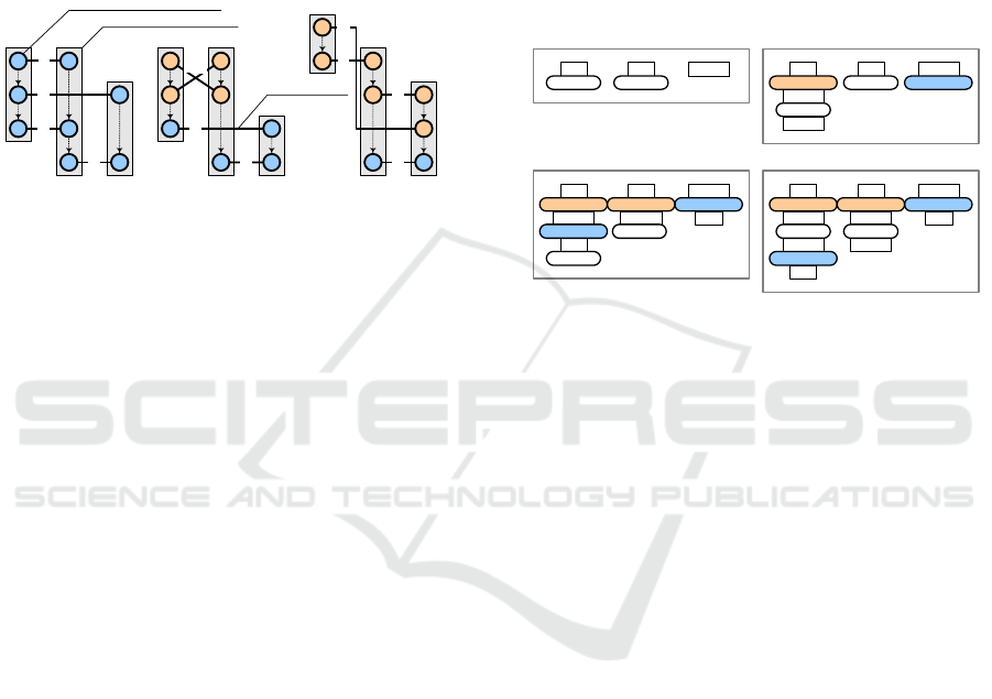
Figure 1: Tangling among robots.
Fig. 1 compares 3 cases related to deadlock
among rendezvous: (1) Not tangled (Fig. 1-a). The
task points of all rendezvouses can be completed
without interfering with each other. No rendezvous-
caused deadlock will occur. (2) Directly tangled
(Fig. 1-b). In this case, we have
∃υ, υ
0
∈ ϒ : ∃π
1
, π
2
∈ υ.Π, π
0
1
, π
0
2
∈ υ
0
.Π
[π
1
, π
0
1
∈ σ
1
, π
2
, π
0
2
∈ σ
2
] :
ι
σ
1
(π
1
) < ι
σ
1
(π
0
1
) ∧ ι
σ
2
(π
2
) > ι
σ
2
(π
0
2
)
indicating a waiting loop that makes schedules not ex-
ecutable: (i) π
1
waits for π
2
(because π
1
, π
2
∈ υ.Π);
(ii) π
2
waits for π
0
2
(because ι
σ
2
(π
2
) > ι
σ
2
(π
0
2
)); (iii)
π
0
2
waits for π
0
1
(because π
0
1
, π
0
2
∈ υ
0
.Π); (iv) π
0
1
waits
for π
1
(because ι
σ
1
(π
1
) < ι
σ
1
(π
0
1
)). (3) Indirectly
tangled (Fig. 1-b). In this case, we have:
∃υ
1
, ..., υ
n
∈ ϒ :
∃π
1,1
, π
1,2
∈ υ
1
.Π, ..., π
n,1
, π
n,2
∈ υ
n
.Π
[(∀i ∈ {2, ..., n} : π
i−1,2
, π
i,1
∈ σ
i
) ∧ π
n,2
, π
1,1
∈ σ
1
] :
(∀i ∈ {2, ..., n} : ι
σ
i
(π
i−1,2
) < ι
σ
i
(π
i,1
)))
∧ ι
σ
1
(π
1,1
) > ι
σ
1
(π
n,2
)
indicating a waiting loop that makes schedules not
executable: π
1,1
waits for π
n,2
which waits for π
n,1
which waits for π
n−1,2
, ..., π
2,1
, π
1,2
, π
1,1
.
3.3 Demand Looping
Assume initially the resource demands of all task
points in the MRS are not satisfied. A straightfor-
ward way to satisfy these demands is to make each
robot to traverse its entire schedule, where for each
task point π whose resource demands π.R
are not
satisfied, the robot will generate a set of rendezvouses
ϒ
prv
(π) to fetch π.R
from stations or other robots.
If no inter-robot coordination strategy is present, an
extreme situation known as demand looping may oc-
cur, in which robots will endlessly “argue” with each
other about who should use the particular set of re-
sources to satisfy itself, without reaching any conclu-
sion. In this section we present two examples to show
the need to introduce inter-robot coordination strat-
egy so as to decide prudently (1) the insertion index
of each rendezvous, and (2) the robot providing re-
quired resources; and the consequences of not to do
so.
Robot h
1
Robot h
2
Station h
3
0 0 knife
1
Robot h
1
Robot h
2
Station h
3
0 0 knife
1-1
knife
Robot h
1
Robot h
2
Station h
3
0 0 knife
1-1-1
knife 0
Robot h
1
Robot h
2
Station h
3
0 0 knife
1-1-2
knife 0
knife
knife
0
knife
0
knife
knife
(a) The initial status of the system, when no robot
has scheduled to obtain the knife
(b) The robot h
1
has scheduled to obtain the knife
(c) In one situation, the robot h
1
gives up the knife
to robot h
2
. If h
2
does the same thing in the next
step, the system will be stuck, with both robots
discussing who will use the knife first.
(d) In another situation, the robot h
1
first uses the
knife, and then give the knife to robot h
2
, which
will satisfy all without causing any infinite loops.
cut◄knife cut◄knife
cut◄knife
cut◄knifeRcv
1
, knife Snd
1
, knife
cut◄knife
cut◄knife
Rcv
1
, knife Snd
1
, knife
cut◄knife cut◄knife
Rcv
1
, knife Snd
1
, knife
Snd
1
, knife
Rcv
1
, knife
Snd
2
, knife
Rcv
2
, knife
Figure 2: A simple case showing demand looping.
Fig. 2 shows the need to constrain the insertion
index of each rendezvous among robots, in order to
prevent the resource demands of one robot from be-
ing sabotaged by rendezvous with another robot. Fig.
2-a shows the initial state. Each robot has a task point
for cutting with a knife. In Fig. 2-b, robot h
1
sets
up the rendezvous for fetching the knife from station
h
3
. Since initially both robots possess no knife, and
there is only one knife, intuitively, h
1
and h
2
must take
turns using the knife, and therefore the ideal next step
would be to let h
2
obtain the knife after h
1
has com-
pleted using it. However, due to the lack of coordina-
tion, in Fig. 2-c, h
2
abruptly schedules to take away
the knife from h
1
without considering h
1
’s need, mak-
ing h
1
unable to complete its schedule. If in the fol-
lowing steps, e.g., Fig. 2-d, they still repeat the same
ruthless decision, then it is possible the rendezvouses
for sending/receiving knife will be repeated for many
times among h
1
and h
2
, while the knife can never have
the chance to be actually used. Note that in order to
prevent this, we can forbid all robot from giving out
resources that are already scheduled to be used by it-
self, i.e., to constrain the insertion of rendezvouses in
the schedules of potential resource providers.
Fig. 3 shows that the MRS must be prudent in
choosing the proper resource provider and receiver
at each step. Fig. 3-a and Fig. 3-b descends from the
same initial status when both robots have no resources
and all resources are in h
3
. Based on different choices
ICAART 2017 - 9th International Conference on Agents and Artificial Intelligence
672

Robot h
1
Robot h
2
Station h
3
0 0 7
1-1
4
1
3
Robot h
1
Robot h
2
Station h
3
0 0 7
1-2
25
4
3
Robot h
1
Robot h
2
Station h
3
0 0 7
1-2-1
25
4
3
1
2
4
1
Robot h
1
Robot h
2
Station h
3
0 0 7
1-2-1-1
25
4
3
1
2
4
1
0
2
2
0
0
Robot h
1
Robot h
2
Station h
3
0 0 7
1-1-1
4 34
0 5
4
3
Robot h
1
Robot h
2
Station h
3
0 0 7
1-1-1-1
4 34
0 5
4
3
2
2
02
1
4
1
2
2
(a) In this case, the robot h
1
accepts resources first
(c) However, robot h
1
soon is forced to give up the
resource to enable robot h
2
to execute
(b) In this case, the robot h
2
accepts resources first
(d) Since it has little consumption, it still can provide
robot h
1
with resources after it has completed
(e) Although also successful, this branch generates
more zigzags which require further processing
0
(f) This branch successfully generated a series of
rendezvouses which satisfy all resource demands
◄4, -3
◄2, 0
◄5, -1
◄3, -1
π
2
π
1
π
4
π
3
Rcv
1
, 4 Snd
1
, 4 ◄4, -3
◄2, 0 ◄5, -1
◄3, -1
π
2
π
1
π
4
π
3
Snd
1
, 5Rcv
1
, 5
◄4, -3
◄2, 0
◄5, -1
◄3, -1
π
2
π
1
π
4
π
3
Snd
1
, 5Rcv
1
, 5
Snd
2
, 2
Snd
3
, 2
Rcv
2
, 2
Rcv
3
, 2
◄4, -3
◄2, 0
◄5, -1
◄3, -1
π
2
π
1
π
4
π
3
Snd
1
, 5Rcv
1
, 5
Snd
2
, 2
Snd
3
, 2
Rcv
2
, 2
Rcv
3
, 2
Snd-4, 1
Rcv
4
, 1
◄4, -3
◄2, 0
◄5, -1
◄3, -1π
2
π
1
π
4
π
3
Rcv
1
, 4 Snd
1
, 4
Snd
2
, 4 Snd
3
, 1
Rcv
2
, 4
Rcv
3
, 1
◄4, -3
◄2, 0
◄5, -1
◄3, -1
π
2
π
1
π
4
π
3
Rcv
1
, 4 Snd
1
, 4
Snd
2
, 4 Snd
3
, 1
Rcv
2
, 4
Rcv
3
, 1
Snd
4
, 2Rcv
4
, 2
Rcv
5
, 2
Snd-5, 2
Snd-6, 1Rcv
6
, 1
Figure 3: The case where initial choices are important.
made at the very first step about who should obtain
the resources first, the system may undergo different
journeys: (1) Fig. 3-a,c,e, shows the branch when h
1
first obtains the resources for its task point π
1
; (2) Fig.
3-b,d,f, shows the branch when h
2
first obtains the re-
sources for π
3
. In Fig. 3-a,c,e, since satisfying π
1
has
used up a lot of resources, leaving no resources for
any other task points of h
1
and h
2
, in Fig. 3-c, h
1
has
no choice but to give up part of its resources and π
1
,
to let others run. In Fig. 3-b,d,f, even after all task
points of h
2
are satisfied, there are still remaining re-
sources in h
1
, h
2
, h
3
, making it possible to satisfy h
1
’s
demands. Although both branches can ultimately sat-
isfying all the resources, Fig. 3-a,c,e branch creates
some zigzags which involve robots planning to deliver
resources forwards and backwards among them with-
out using the resources, due to improper earlier choice
of who would provide and/or receive the resources.
4 ANALYSIS AND SOLUTION
4.1 Prevention of Rendezvous Tangling
Reachable Set of a Rendezvous. We first define
several functions based on reachable sets: (1) the
directly preceding set of rendezvouses ϒ
←
(υ) =
S
π∈υ.Π
Π
(π); (2) the directly succeeding set of ren-
dezvouses ϒ
→
(υ) =
S
π∈υ.Π
Π
(π); (3) the preceding
reachable set of rendezvouses is recursively defined
by ϒ
←
(υ) ⊆ ϒ
←
(υ) and ∀υ
0
∈ ϒ
←
(υ) : ϒ
←
(υ
0
) ⊆
ϒ
←
(υ); (4) the succeeding reachable set of ren-
dezvouses is recursively defined by ϒ
→
(υ) ⊆ ϒ
→
(υ)
and ∀υ
0
∈ ϒ
→
(υ) : ϒ
→
(υ
0
) ⊆ ϒ
→
(υ). The no-
tangling rule can be written as ∀υ ∈ ϒ : ϒ
←
(υ) ∩
ϒ
→
(υ) =
/
0, which is expected to be satisfied by all
the rendezvouses in the schedules at any given time.
In order to ensure there is no tangling, we con-
strain the insertion index of each rendezvous υ when
it is inserted or moved in the schedules. For υ, if
the insertion index ι
σ
(π) of any π ∈ υ.Π has been
specified, ι
σ
(π) poses constraints to the possible in-
sertion indexes of other task points in υ.Π. Assume
Π
in
⊆ υ.Π is the set of task points that have been in-
serted into the schedules without tangling. If we want
to insert one more task point π ∈ υ.Π \ Π
in
without
introducing tangling, its insertion index i in schedule
σ should satisfy the following constraint:
max
υ
0
∈ϒ
←
(υ)
ι
σ
(π
0
) < i ≤ min
υ
0
∈ϒ
→
(υ)
ι
σ
(π
0
)
where {π
0
} = υ
0
.Π ∩ σ 6=
/
0. It can be proven that as
long as the insertion index of any task point of a ren-
dezvous satisfy the above constraint, the no-tangling
rule can always be ensured, and there will be no dead-
lock among robots caused by rendezvous tangling.
4.2 Prevention of Demand Looping
For preventing demand looping, all robots should col-
laborate to determine (1) which robot will generate
the next rendezvous υ for satisfying one of its task
points, (2) which resource holder will provide re-
source for υ. It should prevent the situation of hav-
ing one robot generate all its rendezvouses at one shot
without regarding other robot’s demands. Also, each
robot should consider the degree to which inserting υ
may deprive the chance of the resource provider from
further satisfying its own resource demands. For ex-
ample, if by inserting υ, all further task points would
lost their chances to obtain any resources from any
resource holders, then definitely υ should not be in-
serted, provided there is a better choice.
Crosscut. In order to better depict such thought,
we introduce the concept of crosscut. A crosscut is
a function χ : H → Z, which returns the currently
concerned index in the schedule of each resource
holder. Given a crosscut χ, (1) the set of resources
provided by holder h is R
(h.σ(χ(h))), which shows
Deadlock Prevention in Rendezvous Generation for On-demand Inter-robot Resource Delivery
673

from where other robots can obtain their required re-
sources; (2) the set of resources required by holder
h is R
(h.σ(χ(h))), which is used to compare to the
provided resources R
(h.σ(χ(h))) to see whether χ is
unsatisfied; (3) the preceding crosscut of χ is written
as χ − 1, which is defined as
(χ − 1)(h) =
χ(h) −1 χ(h) > 0
0 otherwise
(4) the succeeding crosscut of χ is written as χ + 1,
which is defined as
(χ + 1)(h) =
χ(h) + 1 χ(h) < |h.σ|
∞ otherwise
(5) we use χ = 0 to represent ∀h ∈ H : χ(h) = 0; (6)
we use χ = ∞ to represent ∀h ∈ H : χ(h) = ∞.
Boundary Crosscut. We define boundary crosscut
χ for depicting the progress of rendezvous generation:
∀h ∈ H :
χ(h) =
i i ≤ |h.σ| ∧ h.σ(1, ..., i − 1)issatisfied
∧ h.σ(i)isnotsatisfied
∞ h.σ(1, ..., |h.σ|)issatisfied
The χ is an upper limit beyond which all task points
are not satisfied. With the rendezvous generation pro-
ceeding, we can imagine a great frontier of satisfied
task points marked by χ gradually pushing forwards
and approaches the ends of all schedules (where χ =
∞), signifying the satisfaction of all task points.
We now make some rules about the process of ap-
proaching χ = ∞ in order to prevent demand looping.
1. The χ and χ should advance to the goal χ = ∞,
and should always choose the way to achieve that
goal with lowest cost.
2. The insertion index of each rendezvous should
be within (χ, χ), so that the task points satisfied
through previous rendezvous planning, should re-
main satisfied in the later rendezvous planning,
and the planning will not omit any task point’s de-
mands nor sabotage any satisfied task points.
3. The task point to be satisfied in the next step of
rendezvous planning should be chosen in such a
way that maximises the opportunity of other task
points to be satisfied in the future planning, so that
entire MRS has the best chance to be all satisfied.
4.3 A*-based Rendezvous Planning
In this section we present a centralised A*-based
Rendezvous Planning Algorithm (ARPA), which tra-
verses all schedules to generate a set of rendezvouses
that satisfy as many task points as possible. The dead-
lock prevention mechanisms shown in Section 4.1 and
Section 4.2 are embedded in ARPA. ARPA can be fur-
ther converted into an equivalent distributed version
in which each robot processes its schedule while per-
sistently communicating with other robots to obtain
information for its own decision-making and to pre-
vent deadlocks (of both types) among robots.
A sub-tree of schedule-level A*-based search
A*-based search(task point level)
0
cc
==
1
,,
m
ii
c
=¥
L
(
)
11
is sati.
sfied
ii
hh
sc
æö
ç÷
è
æö
ç÷
ç÷
èø
ø
Ø
(
)
11
is satisfie
.
d
ii
hh
sc
æö
ç÷
èø
1
1
n
u
11
u
1
1
j
u
… …
…
…
…
1
1
j
u
Generating rendezvous
Inserting a rendezvous
Chosen for its optimality
about total cost, and the
opportunity given to
other task points.
For satisfying
(
)
1 1
.
ii
h
h
sc
æö
ç÷
èø
A*-based search
For satisfying
(
)
(
)
1
1
.h
h
sc
… …
…
()
(
)
1 1
.
h
h
sc
æö
ç÷
èø
¡
prv
Generating rendezvous
A*-based search
For satisfying
(
)
(
)
1
1
1
.
i
h
h
sc
…
()
(
)
1
1 1
.
i
h
h
sc
æö
ç÷
èø
¡
prv
Generating rendezvous
(
)
1 1
.
i i
hh
sc
æö
ç÷
æö
ç÷
ç÷
èø
èø
¡
prv
Generating rendezvous
A*-based search
For satisfying
(
)
122
.
i ii
h
h
sc
æö
ç÷
èø
…
(
)
122
.
iii
hh
sc
æö
ç÷
æö
ç÷
ç÷
è
è
ø
ø
¡
prv
A*-based search
For satisfying
(
)
(
)
1
.
n
n
i
h
h
sc
…
Generating rendezvous
()
(
)
1
.
n
i
n
hh
sc
æö
ç÷
èø
¡
prv
Apply optimal set of rendezvous
(
)
1 1
.
i i
hh
sc
æö
ç÷
æö
ç÷
ç÷
èø
èø
¡
prv
Adapt this set of
rendezvous according to
(
)
1 1
.
i i
hh
sc
æö
ç÷
æö
ç÷
ç÷
èø
èø
¡
prv
Search for next optimal set of rendezvous based on A* algorithm, until it reaches
…
…
…
c
=¥
Update the current crosscut and boundary crosscut
()
1111
,Apply,, .
iiii
hh
c c cc sc
æö
ç÷
ç
æö
æö
ç÷
ç÷
ç÷
èø
ø
÷
èø
è
¡¬
prv
Connected to
other sub-trees
on the
schedule-level
…
…
Figure 4: The search tree of A*-based rendezvous planning
algorithm that combines two granularity levels.
Fig. 4 shows the search tree of ARPA. Assume
initially all robots are without any resources, and all
resources are in the fixed stations. The search begins
with χ = χ = 0, to reach the goal χ = ∞. The search is
divided into two granularity levels: (1) schedule level,
which deals with the goal to make χ = ∞; (2) task
point level, which deals with the sub-goal to satisfy
the demands of each task point.
Schedule Level. In this level, A* algorithm is used
to reach the goal χ = ∞. The algorithm will try
to use the calculation at task point level to satisfy
each task point π on χ, and generate the set of ren-
ICAART 2017 - 9th International Conference on Agents and Artificial Intelligence
674

dezvouses ϒ
prv
(π) which fetch resources for π. Based
on {ϒ
prv
(π) : πis on χ}, it finds the optimal task point
π
∗
:
π
∗
= arg max
πis on χ
f
s
(hϒ
prv
(π
1
), ..., ϒ
prv
(π
n
)i, ϒ
prv
(π))
where f
s
: (P(ϒ))
∗
× P(ϒ) → R is a heuristic fitness
function, which collectively considers following fac-
tors: (1) the cost of completing ϒ
prv
(π); (2) the cost of
previously applied hϒ
prv
(π
1
), ..., ϒ
prv
(π
n
)i; (3) the es-
timated distance from current search step to the goal
χ = ∞, given the current χ and χ; (4) the estimated
influence of applying ϒ
prv
(π) on the opportunities of
other task points becoming satisfied in the future. Af-
ter π
∗
is chosen, it will be put into a frontier set χ
which records all the optimal paths at the schedule
level up to now, and will be the starting point of next
round of schedule-level search. Each node ν
s
of the
search tree at the schedule level is defined as a tuple
hπ, χ, χ
0
, ϒ
prv
(π), ν
←s
i, where (1) π is the task point
to be satisfied by ϒ
prv
(π) (generated by the corre-
sponding task point level search); (2) χ is the cross-
cut reached by ν
s
; all task points before χ will not be
modified by any searches succeeding ν
s
; (3) χ
0
is the
boundary crosscut reached by ν
s
; (4) ϒ
prv
(π) is the
rendezvous sequence generated by the corresponding
task point level search to satisfy R
(π). (5) ν
←s
is the
node that precedes ν
s
in the search tree, from which
we can get the optimal path from χ = χ to ν
s
.
Task Point Level. In this level, A* algorithm is
used to satisfy R
(π) — the demands of each task
point π on χ by finding the best rendezvous sequence
ϒ
prv
(π). The providing task point will be chosen from
the section of crosscuts (χ, χ). At each step, the al-
gorithm will try to insert a new rendezvous into the
ϒ
prv
(π) until R
(π) is fully satisfied. Similar to the
schedule level, in this level, we also choose among
all possible rendezvouses the optimal rendezvous υ
∗
based on the following formula:
υ
∗
= arg max
υ∈ϒ
prv
(π)
f
t
(ϒ
prv
(π), υ)
where f
t
: ϒ
∗
× ϒ → R is the heuristic fitness function
of rendezvous, which is defined similar to f
s
. The
most significant difference is that f
t
considers the dis-
tance to the sub-goal where π is satisfied, rather than
the satisfaction of entire schedule. Each node ν
t
of
the search tree at the task point level is defined as a
tuple hυ, χ, χ, ν
←t
i, where (1) υ is the rendezvous to
be inserted after ν
t
is chosen as optimal; (2) χ is the
crosscut reached by ν
t
; (3)
χ is the boundary cross-
cut reached by ν
t
; (4) ν
←t
is the node that precedes
ν
t
in the search tree, from which we can obtain the
optimal path from ϒ
prv
(π) =
/
0 to ν
t
. The search will
turn to the schedule level when the task point level
search has completed for each task point in χ. In the
task point level, when it is found that currently con-
cerned task point cannot be satisfied without sabotag-
ing other task points, the corresponding search will be
postponed until next round of schedule level search.
5 CONCLUSION
In this paper we analyse the two types of deadlock that
can be introduced into a multi-robot system (MRS) by
uncoordinated generation of resource-delivering ren-
dezvouses among robots. The first type is caused by
rendezvous tangling and is tackled by constraining the
insertion index of each rendezvous according to its
preceding/succeeding reachable set. The second type
is caused by one robot’s resource demands being sab-
otaged by another robot’s rendezvous, and is tackled
by prudent selection of insertion index of each ren-
dezvous and of resource provider/receiver when plan-
ning rendezvouses. We present the sketch of an A*-
based Rendezvous Planning Algorithm (ARPA) that
respects the constraints regarding both types of dead-
lock.
Our future work includes: (1) Determine the spe-
cific form of the fitness functions f
s
and f
t
as speci-
fied in Section 4.3. (2) Conduct an experiment which
shows ARPA can generate efficient and effective ren-
dezvouses for inter-robot delivery. (3) Implement a
distributed version of ARPA with lower computation
and communication cost, which facilitates its applica-
tion on a real-world MRS. (4) Deal with the interac-
tion between ARPA and the rescheduling and reallo-
cating algorithms on MRS.
REFERENCES
Han Lei, Keyi Xing, L. H. F. X. Z. G. (2014). Deadlock-
free scheduling for flexible manufacturing system us-
ing petri-nets and heursitic search. In Computers and
Industrial Engineering, v. 72, n. 1, p. 297-305.
Keshmiri, S. (2011). Multi-robot, multi-rendezvous
recharging paradigm: an opportunistic control strat-
egy. In IEEE ROSE.
Neil Mathew, Stephen L. Smith, S. L. W. (2013). A graph-
based approach to multi-robot rendezvous for recharg-
ing in persistent tasks. In International Conference on
Robotics and Automation.
Neil Mathew, Stephen L. Smith, S. L. W. (2015). Multi-
robot rendezvous planning for recharging in persistent
tasks. In IEEE Transaction on Robotics, v. 31, n. 1, p.
128-142.
Deadlock Prevention in Rendezvous Generation for On-demand Inter-robot Resource Delivery
675
