
Distance-based Live Phylogeny
Graziela S. Ara
´
ujo
1
, Guilherme P. Telles
2
, Maria Em
´
ılia M. T. Walter
3
and Nalvo F. Almeida
1
1
School of Computing, Federal University of Mato Grosso do Sul, Campo Grande, Brazil
2
Institute of Computing, University of Campinas, Campinas, Brazil
3
Department of Computer Science, University of Bras
´
ılia, Bras
´
ılia, Brazil
Keywords:
Evolution, Phylogeny, Live Phylogeny, Neighbor-joining.
Abstract:
The Distance-Based Live Phylogeny Problem generalizes the well-known Distance-Based Phylogeny Problem
by admitting live ancestors among the taxonomic objects. This problem suites in cases of fast-evolving species
that co-exist and are ancestors/descendants at the same time, like viruses, and non-biological objects like do-
cuments, images and database records. For n objects, the input is an n×n-matrix where position i, j represents
the evolutionary distance between the objects i, j. Output is an unrooted, weighted tree where the objects may
be represented either as leaves or as internal nodes, and the distances between pairs of objects in the tree are
equal to the distances in the corresponding positions in the matrix. When the matrix is additive, it is easy
to find such a tree. In this work we prove that the problem of minimizing the residual differences between
path-lengths along the tree and pairwise distances in the matrix is computationally hard when the matrix is
not additive. We propose a heuristic, called Live-NJ, to solve the problem that reconstructs the evolutionary
history based on the well-known Neighbor-Joining algorithm. Results shown that Live-NJ performs better
when compared to NJ, being a promising approach to solve the Distance-Based Live Phylogeny Problem.
1 INTRODUCTION
Distance-Based Phylogeny reconstruction aims at ex-
plaining the evolutionary history of taxonomic objects
and their relations by common ancestors based on the
evolutionary distance between each pair of objects,
which is basically an estimate of the number of chan-
ges that have occurred since they diverged. The goal
is to build an unrooted, weighted tree in which the dis-
tances among leaves – the objects – are equal to the
distances given in the input distance matrix, and the
internal nodes represent hypothetical ancestors.
If the input distance matrix is additive, then it
is possible to find the desired tree in polynomial
time (Felsenstein, 2004; Setubal and Meidanis, 1997).
Otherwise, the problem of minimizing the residual
differences between path-lengths along the tree and
pairwise distances in the input matrix is in the class
of NP-hard problems, i.e. no efficient algorithm for
solving it is known (Day, 1987).
This work addresses the Distance-Based Live
Phylogeny Problem, defined in (Telles et al., 2013),
where living ancestors are allowed to be among the
input objects. Internal nodes in the tree may be either
actual objects (live internal nodes) or hypothetical an-
cestors. Real-world applications include the analy-
sis of viral populations, or other fast-evolving orga-
nisms (Castro-Nallar et al., 2012; Gojobori et al.,
1990; Pompei et al., 2012). Live phylogeny provi-
des different tree topologies, with alternative biologi-
cal hypotheses and shedding light on the relationship
among objects in a population where ancestors and
descendants co-exist. They may also be used in the
analysis of non-biological objects, such as documents
and images, improving mining techniques for data re-
positories (Paiva et al., 2011).
Here we explore computational aspects of the
Distance-Based Live Phylogeny Problem, showing
that the problem is computationally hard. Then we
present a heuristic to solve it, called Live-NJ, based on
the well-known Neighbor-Joining (NJ) method (Sai-
tou and Nei, 1987) for the original distance-based
phylogeny problem. We also apply Live-NJ on a set
of nonadditive matrices, grouped accordingly to three
controlled parameters: the number of objects, the in-
dex of nonadditivity and the number of live internal
nodes. Experiments showed that Live-NJ has better
performance when compared to NJ, seeming to be a
promising approach in trying to solve the Distance-
Based Live Phylogeny Problem.
196
AraÞjo G., Telles G., M. T. Walter M. and Almeida N.
Distance-based Live Phylogeny.
DOI: 10.5220/0006224501960201
In Proceedings of the 10th International Joint Conference on Biomedical Engineering Systems and Technologies (BIOSTEC 2017), pages 196-201
ISBN: 978-989-758-214-1
Copyright
c
2017 by SCITEPRESS – Science and Technology Publications, Lda. All rights reserved
2 DISTANCE-BASED LIVE
PHYLOGENY
The Distance-Based Live Phylogeny Problem takes as
input a symmetric n × n matrix M, where M
i, j
is the
distance between objects i and j. The output is an
unrooted, weighted tree, in which: all internal nodes
have degree 3; each object is represented by a node
(either a leaf or an internal node); and all leaves re-
present objects. Moreover, each path length between
two objects i, j in the tree is equal to M
i, j
.
When it is possible to build such a tree, M is said
to be additive, and the tree is said to be compatible
with M, like in the original Distance-Based Phylo-
geny Problem. Given an additive input distance ma-
trix, it is possible to reconstruct the live phylogeny in
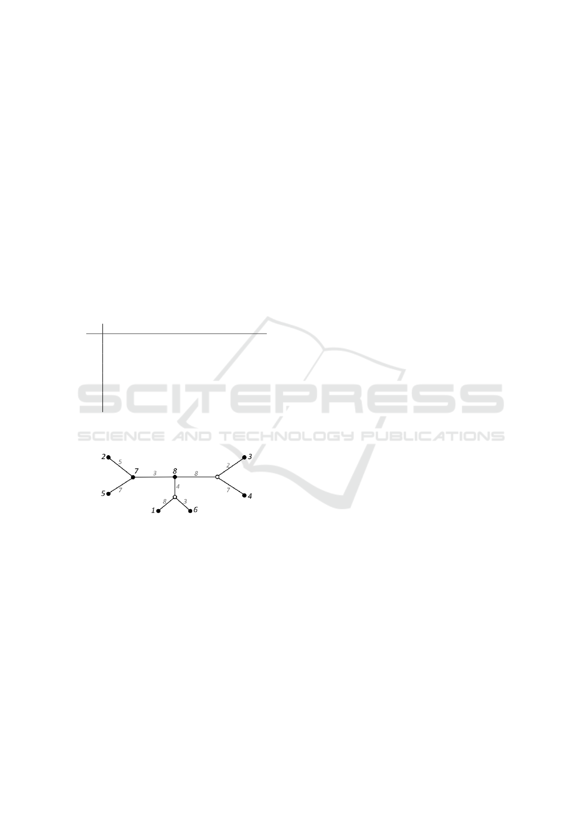
polynomial-time (Telles et al., 2013). Figures 1 and 2
show an additive input distance matrix and the corre-
sponding live phylogeny tree.
1 2 3 4 5 6 7 8
1 0 20 22 27 22 11 15 12
2 20 0 18 23 12 15 5 8
3 22 18 0 9 20 17 13 10
4 27 23 9 0 25 22 18 15
5 22 12 20 25 0 17 7 10
6 11 15 17 22 17 0 10 7
7 15 5 13 18 7 10 0 3
8 12 8 10 15 10 7 3 0
Figure 1: An additive matrix with distances among 8 ob-
jects.
Figure 2: The live phylogeny tree for the matrix in Figure 1.
Input objects 7 and 8 are live internal nodes. Hypothetical
nodes are represented by white circles.
When the input matrix is not additive, the problem
consists in finding a live tree that has the minimum
difference to M. In this section we prove that this
problem is computationally hard, and in Section 3 we
propose a heuristic, called Live-NJ, to solve it.
Starting from a matrix M of pairwise distances
among n objects, the original phylogeny problem is
to build a tree T with exactly n leaves such that the
distances in T better reflects the distances in M. In
the live phylogeny problem we are interested in a tree
that better reflects the distances in M, but having at
most n leaves.
Characterizing the computational hardness of a
problem is important because if a problem is solvable
in polynomial time, then it is probable that a program
will solve it efficiently both in time and in memory
usage. Otherwise it is probably not possible to solve
the problem efficiently in general. Below we show
that the Distance-based Live Phylogeny Problem is
computationally hard by showing that its decision ver-
sion is NP-complete (Theorem 1).
We define Q(M,d) as a measure of the difference
between the distances in M and the distances d in T :
Q =
n
∑
i< j
(M
i j
− d
i j
)
2
. (1)
We also state the following phylogeny decision
problems.
THE DISTANCE-BASED PHYLOGENY PROBLEM (DBPP)
Instance: A matrix M
n×n
and a real number K ≥ 0.
Question: Is there a tree T having exactly n leaves and
edge weights d
i j
, 1 ≤ i < j ≤ n, such that
Q(M,d) ≤ K?
THE DISTANCE-BASED LIVE PHYLOGENY PROBLEM
(DBLPP)
Instance: A matrix M
0
n×n
and a real number K
0
≥ 0 .
Question: Is there a tree T
0
having at most n leaves
and edge weights d
0
i j
, 1 ≤ i < j ≤ n, such
that Q(M
0
,d
0
) ≤ K
0
?
Theorem 1. DBLPP is NP-complete.
Proof. DBPP was shown to be NP-complete by (Day,
1987). We reduce DBPP to DBLPP as part of the
proof that DBLPP is also NP-complete. The re-
duction is trivial: an instance (M,K) of DBPP is
transformed to an instance (M
0
,K
0
) to DBLPP making
M
0
= M and K
0
= K.
If the answer for a DBPP instance is yes, then
there is a tree T with exactly n leaves with weights
d
i j
for each pair i, j such that Q(M,d) ≤ K. It is easy
to see that tree T is also an answer to the DBLPP.
Conversely, if the answer for an instance of
DBLPP is yes, there exists a tree T
0
with weights d
0
i j
for each pair of objects i, j such that Q(M
0
,d
0
) ≤ K
0
.
A corresponding solution for DBPP can be obtained
according to one of the following cases:
• T
0
does not have live internal nodes. Making
T = T
0
gives a tree with exactly n leaves and
Q(M,d
0
) ≤ K, which allows answering yes to
DBPP.
• T
0
has live internal nodes. Build a tree T applying
the following operation while there is a live inter-
nal node in T
0
. Let x be a live internal node repre-
senting object u. Choose an edge (x,z) incident
to x, add a new hypothetical node y splitting this
edge and add an edge connecting y to a new leaf
Distance-based Live Phylogeny
197
node labeled u. Let a be the weight of (x, z). Set
edge weights d
0
xy
= d
0
yu
= 0, and d
0
y,z
= a. Finally,
turn x into a hypothetical node. Figure 3 illus-
trates this operation. When no live internal node
is left, T will have exactly n leaves, and because
pairwise distances in T are the same as those in T
0
by construction, we have Q(M, d) ≤ K. Then T is
answer yes to DBPP.
Figure 3: Transformation of a live internal node u (a) into a
leaf (b) in T
0
. All pairwise distances are preserved.
Thus we may conclude that DBPP polynomially
reduces to DBLPP, and hence DBLPP is NP-hard. It
is straightforward to verify a solution for DBLPP in
polynomial time, and hence DBLPP belongs to NP.
We conclude that DBLPP is NP-complete.
This result improves our understanding on the pro-
blem and signals that, except for small values of n, it
can’t be solved optimally and that we must resort to
near optimal results.
3 LIVE-NJ
NP-complete problems justify the challenge of desig-
ning efficient (polynomial time) heuristics, that is, al-
gorithms that do not guarantee optimal solutions for
every instance of the problem but present good per-
formance. One of the most frequently used heuristic
to solve the original problem of distance-based phylo-
geny (where live internal nodes are not allowed) is the
well-known Neighbor-Joining (NJ) approach (Saitou
and Nei, 1987; Studier and Keppler, 1988). The basic
idea behind NJ is to join, at each step, a pair of ob-
jects that gives the smallest sum of edge lengths. This
chosen pair is joined into a new internal node, and
replaced by this new node before the next step. NJ al-
gorithm is the most popular among the distance-based
methods (Makarenkov et al., 2006).
For the original phylogeny problem, NJ recon-
structs the correct tree when the matrix is additive.
When the matrix is nonadditive, even though there is
no bound to measure the quality of the distances on
the resulting tree, NJ builds the right topology when
the distances in the matrix are sufficiently close to the
true evolutionary distances (Atesson, 1999; Mihaescu
et al., 2009).
For live phylogenies, when NJ receives an additive
matrix as input, it reconstructs a correct tree in terms
of distance, but it does not allocate any object as inter-
nal node. All the objects always appear as leaves. We
show that, for each leaf u in the tree produced by NJ
that should be internal, NJ creates edges with length
zero in the vicinity of u. This is what Theorem 2 sta-
tes. Based on this result, it is possible to make small
changes on that vicinity, promoting u to an internal
live node. This is the core of our heuristic.
Theorem 2. Let M be an additive matrix with at le-
ast 4 objects, T a live tree and T
NJ
an NJ tree, both
compatible with M. For each object u that is an inter-
nal node in T , there are adjacent internal nodes v and
w in T
NJ
such that edges (u,v) and (v, w) have length
zero.
Proof. First suppose that M has exactly four objects.
The tree produced by NJ, T
NJ
, is unique up to relabe-
ling, as shown in Figure 4(a). The live phylogeny T
is also unique, as shown in Figure 4(b).
Figure 4: (a) Phylogeny T
NJ
produced by NJ to four ob-
jects and (b) live phylogeny tree T with four objects. Live
internal node u has degree three.
Since all distances in both trees are compatible
with M, we will call them d. Let u be the internal
node in T . Object u is a leaf in T
NJ
, adjacent to v,
which is adjacent to w, as depicted. From T
NJ
, d
u,t
1
+
d
u,t
2
−d
t
1
,t
2
= 2d
u,v
. By taking distances in T , we have
d
u,t
1
+d
u,t
2
= d
t
1
,t
2
. Thus, d
u,v
= 0. Using a similar re-
lation, in T
NJ
we have that d
u,t
2
+d
u,t
3
−d
t
2
,t
3
= 2d
u,w
,
and d
u,w
= 0.
Now suppose that there are more than four objects.
Then there are three subtrees separated by u, with le-
aves t
1
,t
2
,t
3
,t
4
, as shown in Figure 5. Note that, up
to relabeling, each subtree has at least one leaf, and
one of them has to have more than one leaf. Up to
relabeling, NJ will produce one of the trees shown
in Figures 6 and 7. If NJ produced the tree in Fi-
gure 6, then we have d
u,t
1
+d
u,t
3
−d
t
1
,t
3
= 2d
u,v
. By ta-
king distances in T , we get d
u,t
1
+ d
u,t
3
= d
t
1
,t
3
. Thus,
BIOINFORMATICS 2017 - 8th International Conference on Bioinformatics Models, Methods and Algorithms
198
d
u,v
= 0. Using a similar relation, in T
NJ
we have that
d
u,t
2
+ d
u,t
3
− d
t
2
,t
3
= 2d
u,w
, and d
uw
= 0. If NJ pro-
duced the tree showed in Figure 7, we may apply the
same reasoning to conclude that d
u,v
= d
u,w
= 0.
Figure 5: Live phylogeny tree T with more than 4 objects.
Figure 6: Phylogeny T
NJ
produced by NJ for more than 4
objects, when three objects are gathered in a subtree.
Figure 7: Phylogeny T
NJ
produced by NJ for more than 4
objects, having two objects in two separated subtrees.
Theorem 2 tells us how to use NJ to solve the Live
Phylogeny Problem when the input matrix is additive:
just take each leaf u and internal nodes v,w such that
the lengths of edges (u,v) and (v,w) are equal to zero,
contract both edges making u = w, thus turning u into
a live internal node.
Our Live-NJ heuristic uses the same idea for non-
additive matrices. First it runs NJ. Then, if the input
matrix is additive, it makes all possible contractions
as explained previously to obtain the live tree. If the
input matrix is nonadditive, then there is no guaran-
tee that NJ will produce such well-characterized leaf
u and nodes v,w, as stated in Theorem 2. However,
Live-NJ looks for a leaf u and internal nodes y,z, with
the same topology of u, v, w in the additive case, but
at this time having edges (u, y) and (y, z) with small
lengths, as follows.
Let D be a nonadditive distance matrix with at le-
ast four objects. Let T
NJ
be the tree obtained by NJ,
such that there is a leaf with the configuration shown
in Figure 8, where z, y are hypothetical nodes, and the
lengths a,b,c of the edges incident to y are such that
b,c < a.
After running NJ, our heuristic visits the leaves of
the tree. Let T be the current tree at the beginning
of an arbitrary step of Live-NJ. Take a triple u, y,z,
Figure 8: NJ Tree. Object u is a leaf and b,c < a.
as stated above, if any, and check if the contraction of
edges (u,y) and (y,z) (making z = u and turning u into
a live internal node) creates a tree T
0
better than T , as
shown Figure 9. If T
0
is better than T , we make the
contraction and proceed to the next step, again look-
ing for other triple u, y,z in the same way. Now we
will explain how to calculate the distances in T
0
, in-
cluding length e of the edge (x,u), and how to decide
when T
0
is better than T .
Figure 9: Tree T
0
. After the contraction of edges of T , u
becomes a live internal node.
Calculating distances in T
0
Notice that we replaced edges (x,y),(y, z), (u, y) in T ,
with lengths a,b,c, respectively, by the edge (x,u)
with length e in T
0
.
Let d
0
i, j
be the distance between the objects i and
j in T
0
. In the new tree T
0
, we make e = a + (b +
c)/2 and calculate distances d
0
of T
0
as follows: (i) for
each pair of objects t
1
,t
2
separated by y in T , d
0
t
1
,t
2
=
d
t
1
,t
2
+ (c − b)/2; (ii) for each object t
1
in T , d
0
u,t
1
=
d
u,t
1
+ (b − c)/2; and (iii) for each object t
2
in T ,
d
0
u,t
2
= d
u,t
2
− (b + c). Note that only these distances
change and need to be calculated.
By choosing this kind of subtree, where b,c < a,
and calculating the distances as above, we are trying
to get closer to the situation that we had in the additive
case, i.e., b,c = 0.
Is T
0
better than T ?
Let d
i, j
be the distance between the objects i and j in
T . We measure the variation between distances in D
and in T according to Equation 1.
Tree T
0
is better than T if Q
0
≤ Q + δ, where Q
0
is calculated replacing d with d
0
in Equation 1, and
δ is a parameter that allows Live-NJ to be more or
less strict. If Q
0
≤ Q + δ, we substitute T by T
0
and
continue the process for each remaining leaf, until we
cannot find any triple u, y,z as above, or Q
0
> Q + δ,
for all remaining leaves.
Distance-based Live Phylogeny
199

Complexity
The first step of Live-NJ is to run NJ. The running
time of NJ is O(n
3
). After that, each one of the O(n)
steps of Live-NJ takes O(n
2
) to calculate distances in
T
0
, constant time to verify if a leaf satisfies the condi-
tion stated by Theorem 2 (or, if b, c < a), and O(n
2
)
time to apply Equation 1 to calculate Q
0
. Thus, the
running time of Live-NJ is O(n
3
).
4 RESULTS AND DISCUSSION
In this section we present some preliminary validation
of Live-NJ, comparing its performance with that of
NJ when increasing nonadditivity. By performance
we mean the ability to minimize the score Q(M,d),
according to Equation 1.
The experiments were made using sets of nonad-
ditive matrices, grouped according to three parame-
ters: the number of objects, the index of nonadditivity
(explained below), and the percentage of live inter-
nal nodes. Two datasets have been built: in the first
we assessed the performance of NJ by increasing the
number of objects and the nonadditivity index. In the
second one we assessed the performance of Live-NJ
by increasing the three parameters.
Index of nonadditivity
A distance matrix M is additive only if its set of ob-
jects satisfies the properties of a metric space and also
the 4-point condition (4PC) (Setubal and Meidanis,
1997). In particular, by being a metric space, for any
triple of objects i, j,k, M
i j
≤ M
ik
+ M
k j
. This is the
well-known triangular inequality. 4PC states that, gi-
ven any quadruple of objects, we can label them i, j,
k and l such that M
i j
+ M
kl
= M
ik
+ M
jl
≥ M
il
+ M
jk
.
Let M be a distance matrix. Let α
0
be the number
of triples of M not satisfying the triangular inequa-
lity and β
0
be the number of quadruples not satisfying
4PC. We define the index of nonadditivity I
N
of M as
I
N
= (α
0
/α + β
0
/β)/2, where α and β are the total
number of triples and quadruples of M, respectively.
Notice that 0 ≤ I
N
≤ 1.
Performance assessment
The dataset built to assess the performance of
NJ consists of sets of nonadditive matrices, grou-
ped according to their number N of objects,
N = 10, 20, . . . 100 and their I
N
, in the ranges
(0,0.25],(0.25,0.5],(0.5,0.75],(0.75,1]. For each
value of N and each range of I
N
, a bucket of 100 ma-
trices was built.
Each input matrix is generated by first producing
a random tree, then generating a matrix from the tree.
By construction, such matrix is additive. Then the
matrix is disturbed, basically by choosing a random
triple i, j,k and making M
i j
= M
ik
+ M
k j
+ δ. This
alteration obviously changes α
0
and possibly chan-
ges β
0
, consequently modifying the nonadditivity in-
dex I
N
. For these experiments we used δ = 1.
As expected, the higher is I
N
, the worse the per-
formance of NJ is. Figure 10 shows the variation of
Q(M,d) for the trees built by NJ as I
N
increases, for
10, 50 and 100 objects. Another highlight is that NJ
scores tend to increase faster as N grows.
Figure 10: NJ scores given I
N
, for N = 10,50 e 100 objects.
To evaluate Live-NJ we used the same method
that was used in the evaluation of NJ, but we added
another parameter for the construction of the data-
set: the percentage of live internal nodes. So, be-
sides N and I
N
, we also used the percentage P =
20%,40%,60%,80% of live internal nodes over the
number of leaves. This time the additive matrices
were generated from random trees containing N =
10,20,...100 leaves plus P percent (over N) of live
internal nodes. Thus, for each N = 10, 20, . . . 100, I
N
in (0,0.25], (0.25,0.5], (0.5,0.75], (0.75,1] and
P = 20%,40%,60%,80% over N, a bucket of 100
nonadditive matrices was built.
The results for N = 10, 50 and 100 are shown
in Figures 11, 12 and 13, respectively. Each figure
shows the Live-NJ scores for all values of P. Taking
the same intervals of I
N
, Live-NJ presents a better per-
formance when compared to NJ, even with higher per-
centages of live internal nodes.
BIOINFORMATICS 2017 - 8th International Conference on Bioinformatics Models, Methods and Algorithms
200
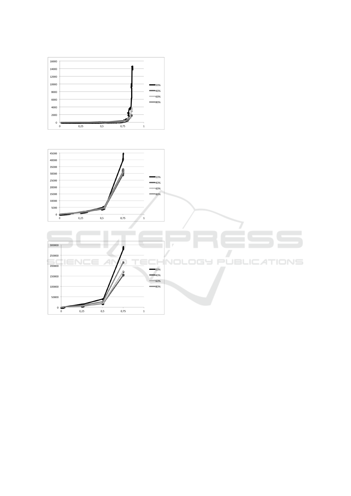
Figure 11: Live-NJ scores given I
N
, for 10 leaves plus P%
of live internal nodes.
Figure 12: Live-NJ scores given I
N
, for 50 leaves plus P%
of live internal nodes.
Figure 13: Live-NJ scores given I
N
, for 100 leaves plus P%
of live internal nodes.
5 CONCLUSIONS
In this article we explored the Distance-Based Live
Phylogeny Problem. We first demonstrated that this
problem is NP-complete. We also presented an NJ-
based polynomial-time heuristic for the problem, cal-
led Live-NJ. This heuristic promotes leaves to internal
nodes, in order to obtain a tree with lower distance va-
riation from the input matrix, simultaneously trying to
build a more realistic topology.
Finally, we applied Live-NJ on a dataset genera-
ted according to controlled parameters: the number
of objects, the index of nonadditivity and the num-
ber of live internal nodes. Experiments showed that
Live-NJ performed better than NJ as the nonadditi-
vity index increases, being a promising approach to
the Distance-Based Live Phylogeny Problem. Next
steps include testing Live-NJ on a real dataset and also
designing new algorithmic solutions for the problem.
ACKNOWLEDGEMENTS
GSA and NFA thank Fundect grants TO141/2016
and TO007/2015. NFA also thanks CNPq grants
305857/2013-4, 473221/2013-6 and CAPES grant
3377/2013. GPT thanks CNPq grant 310685/2015-0.
MEMT thanks CNPq grant 308524/2015-2.
REFERENCES
Atesson, K. (1999). The performance of neighbor-
joining methods of phylogenetic reconstruction. Al-
gorithmica, 25:251–278.
Castro-Nallar, E., Perez-Losada, M., Burton, G., and Cran-
dall, K. (2012). The evolution of HIV: Inferences
using phylogenetics. Mol. Phylog. Evol., 62:777–792.
Day, W. E. (1987). Computational complexity of inferring
phylogenies from the similarity matrix. Bulletin of
Mathematical Biology, 49:461–467.
Felsenstein, J. (2004). Inferring Phylogenies. Sinauer As.
Gojobori, T., Moriyama, E., and Kimura, M. (1990). Mole-
cular clock of viral evolution, and the neutral theory.
P. Natl. Acad. Sci., 87(24):10015–10018.
Makarenkov, V., Kevorkov, D., and Legendre, P. (2006).
Phylogenetic network construction approaches. Bioin-
formatics, 6:61–97.
Mihaescu, R., Levy, D., and Pachter, L. (2009). Why
neighbor-joining works. Algorithmica, 54:1–24.
Paiva, J., Florian, L., Pedrini, H., Telles, G., and Minghim,
R. (2011). Improved similarity trees and their appli-
cation to visual data classification. IEEE Trans. Vis.
Comp. Graphics, 17(12):2459–2468.
Pompei, S., Loreto, V., and Tria, F. (2012). Phylogenetic
properties of RNA viruses. PLoS ONE, 7(9):1–10.
Saitou, N. and Nei, M. (1987). The neighbor-joining met-
hod: a new method for reconstructing phylogenetic
trees. Mol. biol. and evolution, 4(4):406–425.
Setubal, J. C. and Meidanis, J. (1997). Intr. to Molecular
Computational Biology, volume 1997. PWS.
Studier, J. E. and Keppler, K. J. (1988). A note on the
neighbor-joining algorithm of saitou and nei. Mole-
cular biology and evolution, 5(5):729–731.
Telles, G. P., Almeida, N. F., Minghim, R., and Walter, M.
E. M. T. (2013). Live phylogeny. Journal of Compu-
tational Biology, 20(1):30–37.
Distance-based Live Phylogeny
201
