
Multiobjective Optimization using Genetic Programming: Reducing
Selection Pressure by Approximate Dominance
Ayman Elkasaby, Akram Salah and Ehab Elfeky
Faculy of Computers and Information, Cairo University, Giza, Cairo, Egypt
Keywords: Genetic Programming, Multiobjective Optimization, Epsilon Dominance, Evolutionary Algorithms.
Abstract: Multi-objective optimization is currently an active area of research, due to the difficulty of obtaining diverse
and high-quality solutions quickly. Focusing on the diversity or quality aspect means deterioration of the
other, while optimizing both results in impractically long computational times. This gives rise to
approximate measures, which relax the constraints and manage to obtain good-enough results in suitable
running times. One such measure, epsilon-dominance, relaxes the criteria by which a solution dominates
another. Combining this measure with genetic programming, an evolutionary algorithm that is flexible and
can solve sophisticated problems, makes it potentially useful in solving difficult optimization problems.
Preliminary results on small problems prove the efficacy of the method and suggest its potential on
problems with more objectives.
1 INTRODUCTION
Historically, in order to solve optimization
problems, classical search methods were
traditionally used. In every iteration, a single
solution was modified in order to produce better
solutions. However, this point-by-point approach
was overshadowed by the introduction of
evolutionary algorithms(EAs). These algorithms use
the concepts of evolution and natural selection in
optimization. Using populations of individual
solutions, EAs try to capture multiple optimal
solutions for problems lacking one global optimal
solution.
Some optimization, for example industrial,
problems have multiple objectives that need to be
optimized in the same time, which poses extra
difficulties for algorithms that try to solve these
problems. Two main solutions have usually been
followed to reduce the complexities:
Reducing the number of objectives during the
search process or a posteriori during the decision
making process. This approach tries to identify non-
conflicting objectives and discards them.
Propose a preference relation that induces a
finer order on the objective space.
If the aforementioned solutions fail to reduce
multi-objective optimization problems’ complexity,
then the main difficulty facing EAs is incomparable
solutions. Incomparable solutions happen in the
following case. When one solution optimizes one (or
more) objective better than a second solution, but the
second solution optimizes another (or more)
different objective better than the first one.
If we divide the search space into regions based
on how well each solution optimizes each objective,
and assuming no bias towards any region, the
probability of a solution falling into any of these
regions is proportional to the volume of this region
divided by the volume of the entire solution set. As
the number of objectives increases, the number of
regions increases, and the probability that a solution
will fall into a region where one solution optimizes
all objectives efficiently is reduced significantly.
Problems with a large number of objectives,
although apparently similar to problems with less
number of objectives, can’t be solved efficiently
using the same methods used for fewer objectives.
They are computationally more intensive, and
visualizing their solutions becomes harder as more
objectives are added. To avoid these complexities,
some approximate measures are used to obtain good-
enough results of the problem. Epsilon dominance,
notated as ϵ-dominance from now on, is one of these
approximate measures (Laumanns, et al., 2002).
In this paper, genetic programming, a flexible
and powerful type of evolutionary algorithms (EAs),
is used in order to solve optimization problems
424
Elkasaby A., Salah A. and Elfeky E.
Multiobjective Optimization using Genetic Programming: Reducing Selection Pressure by Approximate Dominance.
DOI: 10.5220/0006219504240429
In Proceedings of the 6th International Conference on Operations Research and Enterprise Systems (ICORES 2017), pages 424-429
ISBN: 978-989-758-218-9
Copyright
c
2017 by SCITEPRESS – Science and Technology Publications, Lda. All rights reserved

approximately using ϵ-dominance. We call this
method ϵ-GP. Genetic programming, up to our
knowledge, has not been used before to solve any
optimization problem with an approximate measure.
ϵ-GP is compared to regular genetic programming
(Koza, 1992) in regards to speed, efficiency, and
diversity, and it gives promising results.
The paper is structured as follows. Section 2
explains related work in the field of evolutionary
algorithms. Afterwards, in Section 3 and 4, some
background information is given about optimization
and genetic programming, respectively. An outline
and pseudocode of ϵ-GP are given in Section 5,
while Section 6 deals with the experimentation and
results. Finally, Section 7 contains a conclusion of
the paper and explains future work.
2 RELATED WORK
Evolutionary algorithms have long been successful
in solving MOPs. Schaffer (Schaffer, 1985) started
the movement of EAs solving MOPs by introducing
a vector-evaluated genetic algorithm (VEGA) that
finds a set of nondominated solutions.
Afterwards, the first generation of Multi-
Objective Optimization Evolutionary Algorithms
(MOEAs) started in the early 1990s by using Pareto
ranking and fitness sharing. This generation
consisted of the multi-objective genetic algorithm
(MOGA) (Fonseca & Fleming, 1993), the niched
Pareto genetic algorithm (NPGA) (Abido, 2003)
which is the first algorithm to use tournament
selection, and the nondominated sorting algorithm
(NSGA) (Srinivas & Deb, 1994).
The second generation of MOEAs, which
emerged in the late 1990s and early 2000s,
introduced the concept of elitism (keeping a record
of the best-so-far solutions). It includes the strength
Pareto evolutionary algorithm (SPEA) (Zitzler &
Thiele, 1999) and its improved version(SPEA-2)
which adds a fitness assignment technique, a nearest
neighbor density estimation, and a preservation
truncation method (Zitzler, et al., 2001); the Pareto
archived evolution strategy(PAES) (Knowles &
Corne, 2000); the Pareto envelope based
algorithm(PESA) (Corne, et al., 2000) and its
improved version PESA-II (Corne, et al., 2001 ); and
an improved version of NSGA (NSGA-II) which
splits the pool of individuals into different fronts
according to their dominance and adds a crowding
measure to preserve diversity (Deb, et al., 2002).
NSGA-II is one of the most popular algorithms
in the literature and is usually considered a
benchmark for many new algorithms. This is
because it is very quick in obtaining solutions. It
also yields very efficient results. Although originally
made for problems with smaller number of
objectives, NSGA-II has shown to be somewhat
successful over the years in solving some problems
with more objectives as well.
3 OPTIMIZATION
An optimization problem is a problem where the
goal is to find the best solution from all feasible
solutions for a specific objective function. However,
many of these problems (those that have more than
one objective) exist in a setting that cannot be
expressed using a single function, as different
objectives are usually not measured using the same
metrics.
Furthermore, a multi-objective optimization
problem is defined as simultaneously optimizing
(
)
=
(
)
,….,
(
)
,
(1)
∈
,
by changing n decision variables, subject to some
constraints that define the universe
.
In other words, a multi-objective optimization
solution optimizes the components of
(
)
where
is an n-dimensional decision variable vector =
(
,…,
) from some universe
. Thus, the
problem consists of objectives reflected in the
objective functions, a number of constraints on the
objective functions reflected on the feasible set of
decision vectors
, and decision variables.
In the case of optimizing multiple objectives, it is
usually impossible to find a single solution that
optimizes all of the objectives at the same time. This
gives rise to the definition of nondominated
solutions (also called Pareto-optimal solutions),
which are solutions that optimize some objectives
but are not worse than other solutions in the rest of
the objectives. The Pareto front is the visualization
of all these solutions on the search space. Since
these solutions are nondominated, no one solution
exists that can be said to be better than the other; all
of them are presented to the decision maker as a set
of solutions called the Pareto optimal set.
Multi-objective optimizers usually have to
conform to a few properties; namely, they should
present solutions that are close to the Pareto front as
possible. They should also present different, diverse
solutions to the decision maker that show the
Multiobjective Optimization using Genetic Programming: Reducing Selection Pressure by Approximate Dominance
425
different tradeoffs with respect to each objective.
Optimizers also need to present the best few, which
means that overwhelming the decision maker by
presenting too many solutions is not preferred.
3.1 More Objectives
Optimization problems that have more than 3
objectives are named many-objective optimization
problems, and problems with 2 or 3 objectives are
named multi-objective optimization problems. In
(Khare, et al., 2003), it was found after testing 3
MOEAs from the 2
nd
generation of MOEAs (NSGA-
II, SPEA2, PESA) that these algorithms showed
vulnerability on problems with a larger number of
objectives.
The main difficulties with many-objective
optimization problems are visualization, how to
handle high dimensionality and the exponential
number of points needed to represent the Pareto
front, the greater proportion of nondominated
solutions, and stagnation of search due to larger
number of incomparable solutions. Our work tackles
the latter two difficulties by changing the definition
of dominance to an approximate one, easing the
criteria of acceptance of nondominated solutions.
3.2 Dominance
Multi-objective optimization algorithms insisting on
both diversity and convergence to the Pareto front
face Pareto sets of substantial sizes, need huge
computation time, and are forced to present very
large solutions to the decision maker. These issues
effectively make them useless until further analysis,
because speed and presenting few solutions are very
important to decision makers.
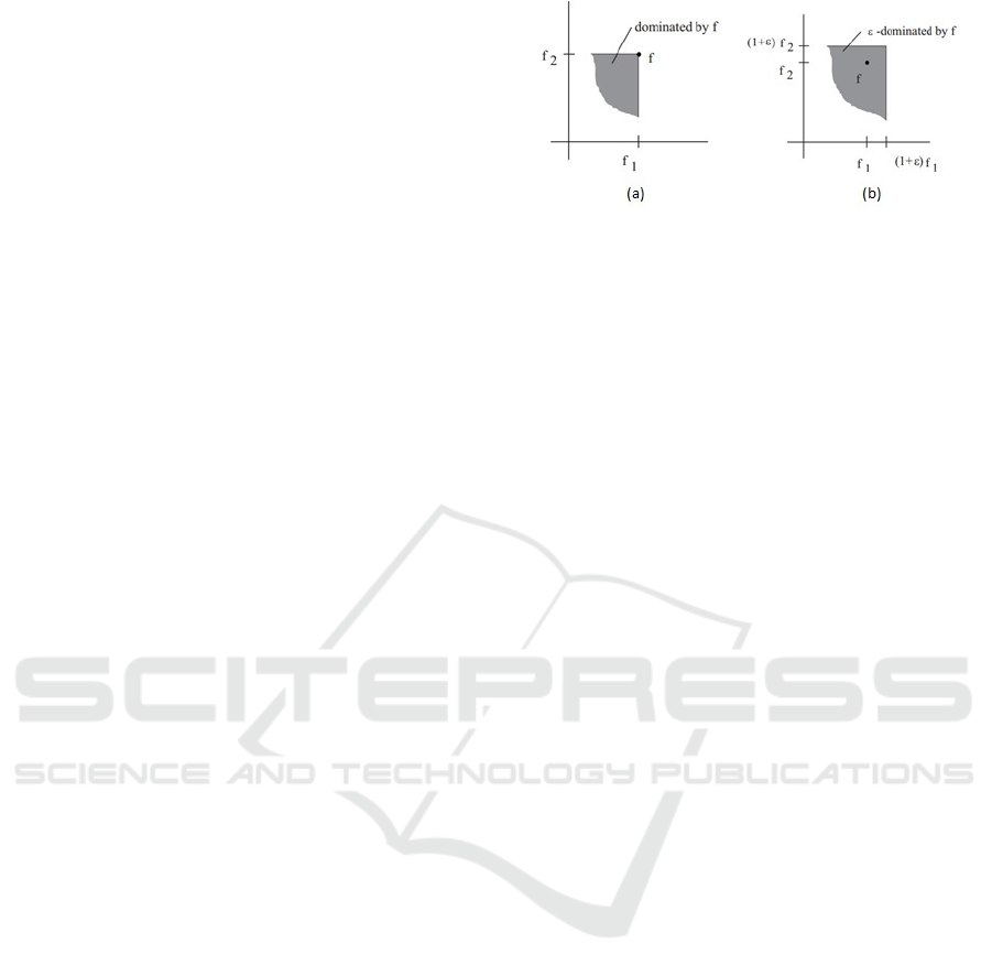
ϵ-dominance (Laumanns, et al., 2002) tries to fix
these problems by quickly searching for solutions
that are good enough, diverse, and few in number. It
approximates domination in the Pareto set by
relaxing the strict definitions of dominance and
considering individuals to ϵ-dominate other
individuals, whereas previously they would have
been nondominated to each other.
In Figure 1, a visual comparison between ϵ-
dominance and regular dominance is shown
(Laumanns, et al., 2002).
4 GENETIC PROGRAMMING
Genetic programming (GP) is one type of
evolutionary algorithms. Its main characteristic is
Figure 1: Differences between (a) regular and (b) ϵ -
dominance.
that it represents solutions as programs (Koza,
1992). This representation scheme is the main
difference between genetic algorithms and genetic
programming. Each solution (program) is judged
based on its ability to solve the problem, using a
mathematical function, the fitness function. Each
program, or solution, is represented using a decision
tree. GP evolves a population of programs by
selecting some candidates that score high on the
fitness function and using regular evolutionary
variation operators on them (mutation, crossover,
and reproduction). New populations are created from
these outputs until any specific termination criterion
is met.
We use strongly-typed genetic programming
(STGP) in this paper, which is one of many
enhanced versions of GP. STGP makes GP more
flexible, explicitly defining allowed data types
beforehand instead of limiting it to only one data
type. Genetic programming, and STGP specifically,
consists of the following.
1) Representation: individuals are
represented as decision trees, but unlike usual GP
(Koza, 1992), STGP doesn’t limit variables,
constants, arguments for functions, and values
returned from functions to be of the same data type.
We only need to specify the data types beforehand.
Additionally, to ensure consistency, the root node of
the tree must return a value of the type specified by
the problem definition and each nonroot node has to
return a value of the type required by its parent node
as an argument.
2) Fitness function: scores how well a
specific execution matches expected results.
3) Initialization: there are two main methods
to initialize a population: full and grow. Koza (Koza,
1992) recommended using a ramped half-and-half
approach, combining the two methods equally.
4) Genetic operators: crossover and mutation.
5) Parameters: maximum tree depth,
maximum initial tree depth, max mutation tree
depth, population size, and termination criteria.
ICORES 2017 - 6th International Conference on Operations Research and Enterprise Systems
426

5 OUR PROPOSED METHOD
Our algorithm, ϵ-GP, has three main characteristics.
First, the performance of our algorithm, and of any
general ϵ-dominance-based MOEA, depends on the
value of ϵ, which is either user defined or computed
from the number of solutions required. Bigger ϵ
values mean quicker computation of solutions, while
smaller values mean solutions that have more
quality. Although the value of ϵ doesn’t have to be
constant for each objective, we make it constant
across all objectives in our method for ease of use
and for quicker computations.
Second, ϵ-GP comprises two storage locations
for solutions:
• An archive that ensures elitism by keeping
the best solutions so far and removing solutions
iff other better solutions are found. We choose to
give this archive a fixed size for several reasons.
One is to limit computation time and to protect
the decision maker from receiving a big number
of nondominated solutions that are
incomparable. Finally, due to ϵ-MOEA
performing well on all test instances in (Li, et al.,
2013), while suffering from archive size
instability, we will stabilize and fix the size.
• A population that stores the current
generation; this current generation can have
worse solutions than a previous generation. This
ensures diversity and keeps us from falling into
local minima.
Third, crossover is always between a solution
from the current generation population and a
solution from the archive. This guarantees both
elitism and diversity. Offspring from crossover are
embedded into the archive if the criteria of
acceptance (to dominate another solution) are met.
They are automatically inserted into the next
generation population as well.
To our knowledge, ϵ-GP is the first algorithm to
combine genetic programming with an approximate
measure, e.g., ϵ-dominance. ϵ-GP uses its
approximation capability to make selection easier
between points by reducing competition and
tolerating a certain additive factor (ϵ) when
calculating dominance. Selection is the most
computation-intensive regular task in Many-O
algorithms, and this is why ϵ-GP is considered
useful.
The initial random generation of the population
and archive in our algorithm is done using the
ramped half-and-half method discussed earlier. The
user inputs in ϵ-GP are the number of runs, the
population size (pop_size), the probabilities G
o
, Pr,
Pc (respectively, probability of a binary or unary
genetic operator, probability of reproduction or
mutation, and probability of crossover).
The pseudocode of ϵ-GP is as follows:
for (i = 0; i < number_of_runs; i++) {
set gen, score to 0; //generation
number
generate pop[gen], archive randomly;
while (score <= minimum_threshold &&
generation < max_generations) {
evaluate fitness of pop[gen];
sort individuals in archive and
pop; // this is where ϵ-dominance is
used
for (j = 0; j < pop_size; j++) {
if (random(0,1) >= G
o
) {
if (random(0,1) >= Pr) {
reproduce (copy) individual;
}
else {
mutate individual;
}
put individual into pop[gen+1];
}
else {
select two individuals from
archive and pop;
if(random(0,1) >= Pc) {
crossover the individuals;
}
else {
reproduce both individuals;
}
j++;//because we insert 2, not
1, individuals
put individuals to pop[gen+1];
}
if (individuals(s) >
archive.worse_result) {
put individual (s) in archive;
score = fitness of archive;
}
Multiobjective Optimization using Genetic Programming: Reducing Selection Pressure by Approximate Dominance
427
}
generation ++;
}
set result[i] to score;
}
6 EXPERIMENTATION
To measure the performance of our algorithm, it was
tested on a basic genetic programming problem: the
ant trail problem (Koza, 1992). Two variants of this
problem are tested; namely, the Santa Fe Trail
problem and the Los Altos Trail problem. The study
used the MOEA Framework, version 2.8, available
from http://www.moeaframework.org/. Koza’s GP
(Koza, 1992) was used as a reference for comparison
in terms of speed and efficiency. We tested the
reference against our algorithm with values of ϵ of
0.1 and 0.01.
We solved each test problem 30 times with
different random seeds. In all runs, no more than
500,000 evaluations were allowed to be made. We
used a crossover probability rate of 0.9, with a point
mutation rate at 0.01. Population size was set to 500.
Since GP is a stochastic algorithm that is affected
by the chosen random seed, it was more suitable to
make a stochastic comparison instead of a static
comparison with the best absolute values. For this
purpose, we analyzed the mean, median, and
standard deviation of the 30 independent runs.
The Santa Fe problem results are shown in Table
1, with better results highlighted in bold when
applicable. The goal is to capture as much pieces of
food as possible, with as little moves as possible. We
also take into consideration how quickly a run
reaches a suitable result.
Table 1: Santa Fe Trail Results.
The results show that our algorithm, ϵ-GP, has
very good performance with regards to all
objectives, and runs quickly as well. At both ϵ
values of 0.1 and 0.01, ϵ-GP has a better average
runtime compared to Koza’s GP, and at ϵ of 0.1, the
food gathered by ϵ-GP is, on average, more than the
food gathered by Koza’s GP.
Next, we test the Los Altos problem, a similar
but harder problem with a more complex trail to
follow to gather the food.
Table 2: Los Altos Trail.
The obtained results, shown in Table 2, prove
that Koza’s GP, while quicker than ϵ-GP, trails ϵ-GP
in both moves and food. ϵ-GP obtained the best
absolute result by eating 129 out of 156 pieces of
food, with 392 moves for ϵ value of 0.01 and 410
moves for ϵ value of 0.1. With an ϵ value of 0.01,
ϵ-GP was very consistent (low standard deviation)
and scored better than the two other sets in both food
and moves, although with a slower running time
than Koza’s GP. Koza’s GP was not able to collect
more than 116 pieces of food, which was achieved
with 335 moves in 2 minutes and 28 seconds. As to
the fastest run, it was achieved by Koza’s GP, where
it collected 52 pieces of food with 493 moves. The
lowest number of moves was achieved by ϵ-GP with
a value of 0.1, where it took 2 minutes and 37
seconds, collecting 55 pieces of food in the process
(the lowest score in all runs).
7 CONCLUSIONS
The previous section shows promising results, as ϵ-
GP was shown to simultaneously optimize two
objectives, with the algorithm guaranteeing
competitive results in all objectives. These results
are encouraging for future work as well, as genetic
programming, up to our knowledge, has never been
used to solve a problem with many (more than 3)
objectives using an approximate measure.
Consistency within stochastic algorithms is
usually a problem due to the random nature of
different runs, but with ϵ-GP with an ϵ value of 0.01,
Mean Median St. De v. Worst Best
Koza 400.533 451 88.1807 494 234
ϵ = 0.1
368.067 366
89.7241
492 226
ϵ = 0.01
380.733 390
85.9386
496 230
Koza 80.3 88 10.3629 55 89
ϵ = 0.1
81.1 89
11.2322 52 89
ϵ = 0.01
80.1 86.5
10.145 57
89
Koza 64.5333 64 8.91621
79 45
ϵ = 0.1
58.5 56.5
8.94331 85
46
ϵ = 0.01
61.7 61
8.78145
81
46
Santa Fe Trail
Variables
Moves
Food
Time
Mean Median St. Dev. Worst Best
Koza 393.7667 414 80.32635
497 221
ϵ = 0.1
402.1 412 81.66346 499 132
ϵ = 0.01
389.667 375 76.2425 498 250
Koza 96.36667 99.5 20.25609 52 116
ϵ = 0.1
99.43333 104 20.6843 55 129
ϵ = 0.01
103.933 115 18.6768 65 129
Koza 142.933 138 22. 27869 191 107
ϵ = 0.1
162.3 159.5 15.803 210 139
ϵ = 0.01
161 150 27.37353 221 129
Variables
Los Altos Trail
Moves
Food
Time
ICORES 2017 - 6th International Conference on Operations Research and Enterprise Systems
428

this is decreased to an acceptable degree. As
problems increase in difficulty, the tolerance of a
high ϵ value starts to decrease and problems can take
longer times to find high-quality solutions and can
face a possibility of falling into local minima due to
the discarding of many solutions. Therefore,
choosing the value of ϵ is very important.
This paper serves as an introduction to further
work that will test ϵ-GP on problems with more than
2 objectives. Furthermore, future work includes the
following:
• The value of ϵ can be input from the user
or dynamically computed. ϵ can also be changed
to be variable for each objective.
• A more detailed study with better test-set
problems that contain more objectives is needed
to prove that ϵ-GP is an efficient many-objective
optimizer;
REFERENCES
Abido, M., 2003. A niched Pareto genetic algorithm for
multiobjective environmental/economic dispatch.
Electrical Power and Energy Systems, February,
25(2), pp. 97-105.
Corne, D. W., Jerram, N. R., Knowles, J. D. & Oates, M.
J., 2001 . PESA-II: Region-based Selection in
Evolutionary Multiobjective Optimization. San
Francisco, s.n.
Corne, D. W., Knowles, J. D. & Oates, M. J., 2000. The
Pareto Envelope-based Selection Algorithm for
Multiobjective Optimization. Paris, s.n., pp. 839-848.
Deb, K., Pratap, A., Agarwal, S. & Meyarivan, T., 2002. A
fast and elitist multiobjective genetic algorithm:
NSGA-II. Evolutionary Computation, April, 6(2), pp.
182-197.
Fonseca, C. M. & Fleming, P. J., 1993. Genetic
Algorithms for multiobjective optimization:
formulation, discussion and generalization. San
Mateo, s.n.
Khare, V., Yao, X. & Deb, K., 2003. Performance Scaling
of Multi-objective Evolutionary Algorithms. Faro, s.n.,
pp. 376-390.
Knowles, J. & Corne, D., 2000. Approximating the
nondominated front using the Pareto Archived
Evolution Strategy. Evolutionary Computation, 8(2),
pp. 149-172.
Koza, J. R., 1992. Genetic Programming: On the
Programming of Computers by Means of Natural
Selection. 1st ed. London: A Bradford Book.
Laumanns, M., Thiele, L., Deb, K. & Zitzler, E., 2002.
Combining Convergence and Diversity in
Evolutionary Multiobjective Optimization.
Evolutionary Computation, September, 10(3), pp. 263-
283.
Li, M., Yang2, S., Liu, X. & Shen, R., 2013. A
Comparative Study on Evolutionary Algorithms for
Many-Objective Optimization. Sheffield , s.n., pp.
261-275.
Schaffer, J. D., 1985. Multiple objective optimization with
vector evaluated genetic algorithms. Pittsburgh, s.n.,
pp. 93-100.
Srinivas, N. & Deb, K., 1994. Multiobjective optimization
using Nondominated sorting in genetic algorithms.
Evolutionary Computation, September, 2(3), pp. 221-
248.
Zitzler, E., Laumanns, M. & Thiele, L., 2001. SPEA2:
Improving the Strength Pareto Evolutionary
Algorithm, Zurich: s.n.
Zitzler, E. & Thiele, L., 1999. Multiobjective Evolutionary
Algorithms: A comparative Case study and the
Strength Pareto Evolutionary Algorithm. Evolutionary
Computation, November, 3(4), pp. 257 - 271 .
Multiobjective Optimization using Genetic Programming: Reducing Selection Pressure by Approximate Dominance
429
