Distributed In-network Processing of k-MaxRS in Wireless Sensor

Networks

Panitan Wongse-ammat

, Muhammed Mas-ud Hussain

, Goce Trajcevski

Besim Avci

and Ashfaq Khokhar

Department of Electrical Engineering and Computer Science, Northwestern University, Evanston, U.S.A.

Department of Electrical and Computer Engineering, Illinois Institute of Technology, Chicago, U.S.A.

Keywords:

k-MaxRS, Maximizing Range Sum, Distributed Query Processing, Wireless Sensor Networks.

Abstract:

We address the problem of in-network processing of k-Maximizing Range Sum (k-MaxRS) queries in Wireless

Sensor Networks (WSN). The traditional, Computational Geometry version of the MaxRS problem considers

the setting in which, given a set of (possibly weighted) 2D points, the goal is to determine the optimal location

for a given (axes-parallel) rectangle R to be placed so that the sum of the weights (or, a simple count) of the

input points in R’s interior is maximized. In WSN, this corresponds to ﬁnding the location of region R such

that the sum of the sensors’ readings inside R is maximized. The k-MaxRS problem deals with maximizing

the overall sum over k such rectangular regions. Since centralized processing – i.e., transmitting the raw read-

ings and subsequently determining the k-MaxRS in a dedicated sink – incur communication overheads, we

devised an efﬁcient distributed algorithm for in-network computation of k-MaxRS. Our experimental obser-

vations show that the novel algorithm provides signiﬁcant energy/communication savings when compared to

the centralized approach.

1 INTRODUCTION

Wireless Sensor Networks (WSN) consist of hun-

dreds, or even thousands of nodes capable of sensing

particular set of phenomena, performing basic com-

putations and, most importantly, communicating with

each other (Akyildiz et al., 2002). They are the em-

powering technology for a wide range of applications

including environmental monitoring, smart buildings

and cities, safety and hazard detection, agriculture,

medicine, military, trafﬁc monitoring, etc. Due to the

types of sensors used and/or various deployment con-

straints (e.g., harsh and inaccessible environments),

re-charging nodes’ batteries is not always feasible.

Consequently, reducing the energy consumption is an

ever-important topic in WSN, facilitating an exten-

sion of overall network’s operational lifetime (Anas-

tasi et al., 2009). While periodic sampling and trans-

mission to a dedicated base-station may be applica-

ble for certain applications, they may incur signiﬁ-

cant overhead in others – especially in event-based

monitoring and tracking. To minimize communi-

cation overheads, various works have tackled cou-

pling of routing schemes with aggregation and in-

network query processing (Fasolo et al., 2007; Krish-

namachari et al., 2002; Trigoni and Krishnamachari,

2012; Madden et al., 2005).

In this work, we take a ﬁrst step towards providing

a distributed, energy-efﬁcient solution in WSN set-

tings, to the problem known as (k-)MaxRS – which

can be described as follows. Given a collection of

weighted objects O and a rectangle R with ﬁxed di-

mensions (i.e., d

× d

), the Maximizing Range Sum

(MaxRS) query retrieves the location at which (the

centroid of) R should be placed, so that the sum of

the weights of the objects in its interior is maximized.

In the context of WSNs, we can think of the set of

sensor nodes as the set of weighted objects, where

the “weights” are application dependent, e.g., mote

readings (event monitoring), information gain (track-

ing an object), uniform (counting), etc. We note that

MaxRS is rather different from the traditional range

query in the sense that when processing a range query,

the region is typically ﬁxed and one is interested in

properties that hold in its interior. Contrary to this,

MaxRS determines where should a rectangle with

given dimensions be placed, so that some “interest-

ing” properties in its interior are maximized (modulo

all the other possible placements). An instance of the

MaxRS in WSN is shown in Figure 1(a), assuming

108

Wonge-ammat P., Mas-ud Hussain M., Trajcevski G., Avci B. and Khokhar A.

Distributed In-Network Processing of k-MaxRS in Wireless Sensor Networks.

DOI: 10.5220/0006210701080117

In Proceedings of the 6th International Conference on Sensor Networks (SENSORNETS 2017), pages 108-117

ISBN: 421065/17

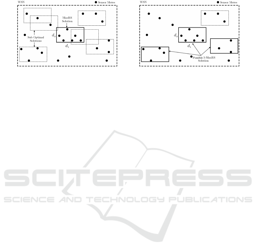
(a) (b)

Figure 1: An example of (a) MaxRS and (b) k-MaxRS problem in WSN.

that the weights of all the sensor nodes are uniform –

i.e., the “counting” variant.

Consider the following query:

Q1: “Where should we place k surveillance devices

(e.g., cameras, checkpoints, etc.) with a ﬁxed-size

coverage region in a forest such that their cumula-

tive monitoring of forest-ﬁre vulnerable regions (i.e.,

regions where temperature and light sensor readings

are higher) is maximized?”.

It is not hard to adapt Q1 to other applications

in which a simultaneous detection of top-k “popu-

lar” regions (k ≥ 2) may be of interest. Such ex-

amples are: discerning k herds of tracked animals

(e.g., gazelles) with largest density; aiding trans-

portation system management by identifying k re-

gions of the city with heaviest trafﬁc; detecting con-

gestions/hotspots in WSN by setting a node’s cur-

rent incoming/outgoing network trafﬁc as its weight.

One can also readily extrapolate to various collabora-

tive scenarios – e.g., guiding drones towards regions

where certain phenomenon has the largest weighted

sum. To the best of our knowledge, the existing solu-

tions (Hussain et al., 2015) to MaxRS queries in WSN

can only be applied to retrieve an optimal location for

a single rectangle R, whereas Q1 is an instance of the

k-MaxRS variant – which we tackle in this work.

The respective k-MaxRS query ﬁnds the

placement-locations for k rectangles such that

the weighted sums of all the objects in the (union of

the) interiors of each of R placed at those locations are

optimal. An example-solution of the k-MaxRS query

in WSN for uniformly weighted nodes is illustrated

in Figure 1(b) (k=3). Although the MaxRS problem

has been addressed by both computational geometry

and spatial databases communities (Choi et al., 2012;

Choi et al., 2014; Imai and Asano, 1983; Nandy and

Bhattacharya, 1995), to the best of our knowledge,

there has been no solution considering k optimal

placements in WSN settings. As mentioned, in

WSNs it is paramount to have energy-efﬁcient query

processing, for which in-network aggregation of

partial results is often the approach of choice (Fasolo

et al., 2007; Krishnamachari et al., 2002). Another

challenge in this scenario is that the weights (i.e.,

sensor readings, information gain, etc.) of the sensor

nodes may change with time, although their locations

are ﬁxed.

The main contribution of this paper can be sum-

marized as follows:

• We provide an efﬁcient in-network distributed algo-

rithm to compute k-MaxRS via a hierarchy of clusters.

• We provide effective data-sharing schemes among

the cluster-heads (also called principals).

• We provide experimental observations quantifying

the beneﬁts of the proposed approach.

The rest of the paper is organized as follows: Sec-

tion 2, introduces the necessary technical background

and presents the formal description of the k-MaxRS

problem. In Section 3, we discuss in details the pos-

sible centralized approaches and the different compo-

nents of our distributed solutions. Section 4 presents

the quantitative observations of the beneﬁts of our ap-

proaches and Section 5 positions this work with re-

spect to the related literature. We conclude the paper

and outline directions for future work in Section 6.

2 PRELIMINARIES

We now introduce the basic notation, followed with

an overview of the MaxRS problem and formal

deﬁnition of the k-MaxRS query in WSN. We also

brieﬂy describe the existing solutions for the MaxRS

problem to better motivate the algorithms and imple-

mentations proposed in this paper.

We assume a WSN covering an area

W SN

= l × w and consisting of n nodes, i.e.,

WSN = {sn

,sn

,. .. ,sn

}, where each sn

equipped with whatever sensors are appropriate for

the phenomena of interest for a given application.

In addition, we also assume that the WSN is dense

Distributed In-Network Processing of k-MaxRS in Wireless Sensor Networks

109

enough to ensure a coverage (i.e., every location in

W NS

is within the sensing range of at least one node)

and connectivity (i.e., every two nodes sn

and sn

can communicate with each other either directly or

via multiple hops).

MaxRS: Let C(p,R) denote the region covered by R

centered at a particular point p. We have:

Deﬁnition 1. (MaxRS) Given a set of n points O =

,. .. o

}, and each o

associated with a weight

, the MaxRS query retrieves a position p within the

given space for an isothetic rectangle R of size d

×d

such that

∑

∈ O ∩C(p,R)}

is maximal.

In case of ties, one position is selected arbitrarily

as the MaxRS solution. Without loss of general-

ity, we assume that the set of points/objects O =

,. .. ,o

} coincides with the set of nodes in the

WSN = {sn

,sn

,. .. ,sn

}. The weight(s) associated

with a sensor node can be determined based on the

various readings, as needed by a speciﬁc application.

k-MaxRS: Let Interior(p,R,O) denote a function that

returns the subset of objects from O contained within

R, when the centroid of R is placed at a given point p.

Deﬁnition 2. (k-MaxRS) Given a set of n points O

= {o

,. .. o

}, each o

associated with a weight w

and an integer k ≥ 2, the k-MaxRS problem ﬁnds a

set of locations P = {p

, p

,. .. p

} for the centroids

of k isothetic rectangles R

, R

,. .. , R

, each of size

× d

such that:

1. For each p

∈ P,

∑

∈ O ∩C(p

)}

≥

∑

∈ O ∩C(p

)}

, ∀p

/∈ P

2. Interior(p

,R, O) ∩ Interior(p

,R, O) =

∀p

, p

∈ P and p

6= p

The second condition of the deﬁnition ensures

that there are no overlapping objects between any

two top-k solutions of the k-MaxRS problem. We

note that, just like in the case of MaxRS, there can

also be multiple possible solutions for the k-MaxRS

problem as shown in Figure 1(b) – another rectangle

(dashed) can also be taken as part of the solution, in

place of the bottom right one.

In-memory MaxRS Solution: To compute MaxRS

for static objects with ﬁxed weights, the problem is

initially transformed into a “dual” rectangle intersec-

tion problem as follows (cf. (Nandy and Bhattacharya,

1995)). For simplicity, let us consider the counting

variant of the MaxRS problem here. We ﬁrst draw a

rectangle of size d

× d

centered at each of the ob-

jects in O. R covers o

if and only if its center is in

the interior of the dual rectangle of o

. Thus a rect-

angle covering the maximum number of objects can

be centered at any location within the maximum in-

tersecting region of the dual rectangles. Using the

ﬁndings of (Imai and Asano, 1983) and this trans-

formation, (Nandy and Bhattacharya, 1995) provided

an in-memory algorithm to solve the MaxRS problem

in O(n logn) time. Considering the top and bottom

edges of the rectangles as horizontal intervals, an in-

terval tree – i.e., a binary tree on the intervals – is con-

structed, and subsequently a horizontal line is swept

in a bottom-up manner. The algorithm maintains the

count for each interval currently residing in the tree,

where the count of an interval represents the num-

ber (or, the sum of weights) of overlapping rectangles

within that interval. An interval with the maximum

count during the whole sweeping process is the ﬁnal

solution.

3 PROCESSING k-MaxRS

We start this section with presenting two techniques to

compute k-MaxRS in centralized settings: Object Re-

moval Method (ORM) and List Method (LM). This

is followed by the details of our proposed in-network

algorithm for processing k-MaxRS that employs clus-

tering, routing, and data-aggregation schemes.

3.1 Centralized Algorithms for

k-MaxRS Processing

Objects Removal Method (ORM): The sim-

ple/intuitive idea behind this method is to use the

MaxRS algorithm (Nandy and Bhattacharya, 1995) it-

eratively k times, as follows:

1. Execute the MaxRS procedure over the current set

of objects, and retrieve the optimal location p for

the query rectangle R.

2. Set the current set of objects to be O −

Interior(p,R).

After performing steps (1) and (2) k times and

storing the solution from each iteration, we can

obtain the answer-set to the k-MaxRS problem. Since

MaxRS solution in (Nandy and Bhattacharya, 1995)

takes O(n log n) time, the overall complexity of this

technique is O(kn logn).

List Method (LM): This is a modiﬁed plane-sweep

procedure based on (Nandy and Bhattacharya, 1995),

where each internal node v of the interval tree main-

tains a ﬁeld target – pointing to the interval with max-

imum count within the sub-tree rooted at v itself. To

compute k-MaxRS, we maintain an answer-set of size

k during the whole plane-sweep procedure. Whenever

SENSORNETS 2017 - 6th International Conference on Sensor Networks

110

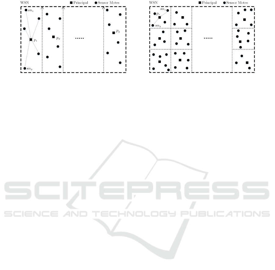
(a) (b)

Figure 2: Different types of clustering schemes: (a) vertical slabs (b) m × n grids.

a new interval (a.k.a. window) is added to or removed

from the tree, the target pointers of the affected in-

ternal nodes are updated accordingly. When an inter-

val is inserted/deleted – only a subset of the interval

tree is affected (all the nodes in path F

, F

, and F

– cf. (Nandy and Bhattacharya, 1995)). Thus, after

insertion/deletion of an interval, the answer-set is up-

dated by comparing with the target values of these af-

fected nodes only. All such nodes can be traversed in

O(logn) time, and O(k) time is needed to update the

answer-set for a changed target value. The processing

time of a single plane-sweep event is thus O(k log n).

As there are O(n) events (2 for each rectangles, i.e.,

top and bottom edges), the time-complexity of this al-

gorithm is O(kn logn).

Additionally, suppose two intervals I

and I

over-

lap, and count(I

) ≥ count(I

). In such cases, I

would

be discarded from the answer-set even if its count puts

it in the top-k (due to violation of condition 2 of Def-

inition 2). Note that, we maintain a hash-table, dict,

where a key is an interval and corresponding value is

a set of intervals that have been discarded from con-

sideration due to overlapping with the key interval. If

we consider the previous example, one of the <key,

value> pair of the dict table will be < I

, {I

} >. This

aids us in retrieving the interval I

back, if later I

itself

is discarded for overlapping with another interval of

higher count. As we use a hash-table (i.e., amortized

access cost of O(1)), this does not affect the overall

time-complexity.

Extension & Comparison

Both LM and ORM can be used to process k-MaxRS

in WSN in a na

ıve manner, i.e., all the sensed values

(or, current weights) are transmitted to the sink (di-

rectly or via multi-hop transmission), where the sink

can use either of the two techniques to compute cur-

rent MaxRS solution. ORM has two signiﬁcant pit-

falls:

• Firstly, it can still produce answer-sets violating

condition 2 of Deﬁnition 2.

• Secondly, and more importantly, for some degen-

erated cases, it can produce sub-optimal k-MaxRS

answer-sets.

Regardless of these, though, any centralized process-

ing which takes place in a dedicated sink incurs a sig-

niﬁcant communication overhead.

3.2 Distributed Algorithm for k-MaxRS

Processing

The basic idea behind our proposed in-network pro-

cessing is: (1) Divide the whole network into sub-

networks (clusters); (2) Localize the computation pro-

cess within the clusters; and (3) Execute a data ag-

gregation scheme between neighboring clusters – the

details of which we present in the sequel.

Geographical Clustering

In (Choi et al., 2014), a distributed solution to

the MaxRS problem was devised for large spatial

databases, extending the idea of the in-memory algo-

rithms to the settings in which data resides on a sec-

ondary storage. The work aimed at reducing the num-

ber of I/O’s – and the main idea was centered around

dividing the space into m vertical slabs along the X -

dimension, until the number of rectangles in a slab

can ﬁt in the main memory. For each slab, a variant

of the in-memory sweep-line algorithm is performed

and the results are saved in a slab ﬁle. Finally, all the

local slab ﬁles are merged into one solution slab ﬁle.

Although the idea works well in spatial databases con-

text, its straightforward extension is not well-suited in

case of WSN. A vertical subdivision of a sensor net-

work (similar to (Choi et al., 2014)) is presented in

Figure 2(a). Each such slab (cluster) is assigned a

local principal (similar to cluster-heads), which is in

charge of gathering the raw data (i.e., weights) from

all the nodes in the interior of its own slab. As the

sensor ﬁeld can be of a large size in both length and

width, some sensor nodes might still be far from the

Distributed In-Network Processing of k-MaxRS in Wireless Sensor Networks

111

local principal which will result in inefﬁcient network

route to that principal – e.g., path to p

from nodes

and sn

in Figure 2(a).

To avoid such cases, we propose to split the zone

of interest into m × n grid of equal-sized cells. Each

cell will be assigned a local principal, and the value of

m and n can be set based on some desired criteria, e.g.,

the average number of sensors within a cell, a limit

on the number of hops when communicating with the

principal, etc. The beneﬁt of this space-clustering

method is shown in Figure 2(b), as now we can con-

trol the communication distance between nodes and

their local principal. Other similar space-partitioning

schemes (e.g., K-d tree (Mohamed et al., 2013)) can

be considered, but the important observation is that

subsequently the principals are organized in a hierar-

chical (tree-like) digraph – principal graph – rooted

in a dedicated sink (more details in the following sec-

tions). The impact of this geographic clustering and

hierarchical digraph for principals is two-fold: (1) It

helps in localizing the processing as each principal

can compute k-MaxRS for its own cell; and (2) It en-

ables a distributed solution even for the case when

some of the rectangles from the k-MaxRS answer-set

spans across ≥ 2 cells.

Base Method

For in-network processing, LM is more suited than

ORM, because ORM would need to execute MaxRS

k times iteratively, and doing the in-network process-

ing k times among the clusters would still incur sig-

niﬁcant communication overhead – possibly even ex-

ceeding the centralized approach for a large k. On

the other hand, the sweep-line procedure is performed

only once for LM, i.e., a single in-network process-

ing cycle can retrieve the k-MaxRS answer-set. Thus

in our distributed technique, each local principal in a

given cluster uses LM to compute the answer-set in

that cluster.

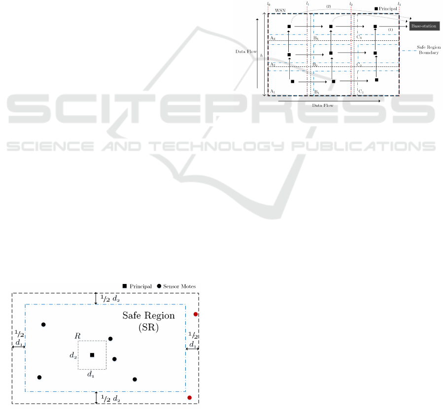
Routing & Data Aggregation

One way to divide routing protocols in WSN is into

Figure 3: The safe region within a cell.

two categories: hierarchical and “ﬂat”. In this work,

we employ a hierarchical digraph-based routing pro-

tocol among the principals, and data propagation and

aggregation is achieved by relaying messages from

predecessors to successors. As a result, the local prin-

cipals form a digraph, denoted principal graph, in

our distributed scheme. Before going into the details

about principal graph, we deﬁne the term safe region

(SR) for a cell as the geographical region within which

all the local processing of k-MaxRS for that cell is ﬁ-

nal. In other words, no k-MaxRS solution can span

outside the safe region. The safe region of a cell for

a given query rectangle R of size d

× d

is illustrated

in Figure 3, and we observe that the information of all

the sensor nodes 6∈ SR (indicated in red in Figure 3)

must be shared with the neighboring cells when de-

termining the answer.

Figure 4: The principal graph and data aggregation to the

sink.

A cell can have as many as 8 neighbors (e.g., B

in Figure 4), and sharing data with all of them may

not be efﬁcient. Instead, we use the principal graph as

shown in Figure 4. For a principal p

of the cell M

(under a suitable cell-addressing scheme), we will use

and p

to denote the set of its predecessors and

successors in the principal graph respectively. The

hierarchical digraph is formed by creating directed

edges from each principal to the principals of the cells

immediately up (“north”) and right (“west”) direc-

tions (if exists). Thus, a principal will have at most

two successors and two predecessors in the graph,

e.g., for A

in Figure 4 – p

={A

} and p

={A

Successors are considered to be in higher level in the

hierarchy than their predecessors, and the sink is kept

in the highest level of the hierarchy (i.e., has no suc-

cessors). In this scheme, each principal p

shares its

data with only at most two neighbors – its successors,

i.e., p

. Thus, p

in Figure 4 will share its data with

only p

and p

. A principal shares the following

data with its successors: (1) local k-MaxRS answer-

set; (2) the dict hash-table; and (3) the data of the

nodes in the unsafe region. In this setting, the prin-

cipal of cell A

has the valid k-MaxRS answer-set for

the region of the network between l

and l

(cf. Fig-

SENSORNETS 2017 - 6th International Conference on Sensor Networks

112

ure 4). Similarly, the principal of cell B

has valid

answers for the region l

and l

, and so on. Finally,

the sub-solutions can be merged in two ways: (1) In

the top-right cell (i.e., C

in Figure 4); and (2) In the

base-station (using dotted connections in Figure 4).

To eradicate any dependency on the base-station, we

employ the former method.

Algorithms

There are two types of nodes (entities) in our dis-

tributed scheme: (1) Sensing nodes; and (2) Local

principals. The behavior of a sensing node in k-

MaxRS processing is rather simple:

1. After a pre-determined (ﬁxed) period, col-

lect/update its own application-speciﬁc weights

(e.g., sensed phenomena values, network trafﬁc,

consumed energy, etc.).

2. If there is any update of the weight, send the new

value to the local principal.

The behavior of local principals is speciﬁed in Al-

gorithm 1, which we now explain. Initially a prin-

cipal receives the cell-boundary information, along

with two other values – (1) the dimensions of the

range R; and (2) λ – the re-evaluation frequency –

directly from the base-station. Using the received

parameters, the principal establishes connection with

Algorithm 1: k-MaxRS-Principal (R, λ, C).

Require: A rectangle R of size d

× d

, a time-

interval λ, and a principal’s own cell C

Ensure: Sending data to be shared with p

, or the

ﬁnal answer-set kmaxrs to the sink

1: Establish connection with all sn

∈ WSN

2: Establish connection with p

and p

3: Compute safe region SR using C and R

4: while Not Interrupted do

5: Receive (location, w

) data from all sn

∈

WSN

6: Receive (kmaxrs

,dict

,unsafe

) from p

∈ p

7: if a time-interval ends after λ time then

8: Add unsafe

to WSN

9: (kmaxrs,dict) ← LM(WSN

,R)

10: Merge dict and dict

from p

∈ p

11: kmaxrs ← Compare(kmaxrs, kmaxrs

dict)

12: if p

={sink} then

13: return kmaxrs to the sink

14: else

15: return (kmaxrs,dict,unsafe) to p

16: end if

17: end if

18: end while

the relevant nodes, i.e., all the nodes in its cell, and

the principals corresponding to its p

and p

neigh-

bors (cf. Lines 1-2). SR is then computed and the

principal detects/marks the nodes in its unsafe region

(Line 3). Lines 5-17 are executed until new param-

eters are received from the base-station. In Lines 5-

6, the principal waits to receive relevant information

from the sensing nodes (i.e., the weights of their mea-

surements), and p

. At each time-interval λ, Lines

8-16 are processed. After adding the information of

nodes in the neighboring predecessor principals’ un-

safe regions, a principal performs the LM method to

compute its own local k-MaxRS answer-set (cf. Lines

8-9). Then it combines the dict tables from the neigh-

bors with its own in Line 10. In Line 11, Compare is

a method which takes all the local solutions – a cell’s

computed answer-set and from p

– and retrieves the

top-k non overlapping positions using the merged dict

hash-table. Finally, if the principal is the immediate

predecessor of the sink, it sends the ﬁnal solution only

directly to the sink. Otherwise, relevant information

is sent to p

We re-iterate that there is the user-deﬁned param-

eter λ (a.k.a. sampling rate) specifying the “fresh-

ness” of the answer-set, i.e., the frequency of re-

evaluating k-MaxRS. What this entails is if k-MaxRS

is computed at time t, only the nodes within the

answer-set rectangles are kept awoken between t and

t +λ, thereby limiting the awareness of the ﬂuctuation

of the weights corresponding to the monitored phe-

nomenon. At time t + λ, all nodes are awakened, and

subsequently k-MaxRS is re-computed with updated

weights throughout the entire network and the states

(awake, or idle) of the nodes are changed accordingly.

4 EXPERIMENTAL EVALUATION

We now describe our experimental observations re-

garding the beneﬁts of the proposed approaches

Tools and Setup: We conducted the experi-

ments in an open-source WSN simulator, SIDnet-

Swans (Ghica et al., 2008) – which has been used

as an experimental tool in prior works (Trajcevski

et al., 2011; Bai et al., 2011). The simulator is con-

ﬁgured as follows: (1) 20 Kbps radio data rate on

the MAC 802.15.4 protocol; (2) Shortest path geo-

graphical routing algorithm protocol (Banerjee et al.,

2012) between nodes; (3) Utilization of Heart-Beat

protocol (Li and Tan, 2007) to create the routing ta-

ble in the MAC layer for each node within the ﬁrst

All the source codes and datasets for the experi-

ments reported in this paper are publicly available at:

http://www.eecs.northwestern.edu/˜pwa732

Distributed In-Network Processing of k-MaxRS in Wireless Sensor Networks

113

(a) (b)

Figure 5: (a) Hop count comparison, and (b) Amount of packet loss between centralized and distributed schemes.

Figure 6: Hop count comparison between different dis-

tributed schemes.

hour when the simulation starts; (4) Communication

range of 100 meters; (5) Power consumption model

according to the TelosB mote’s speciﬁcations; and

(6) Initial capacity of a fully-charged battery of 25

mAh. Note that, a fully-charged sensor can run for 48

active-hours during simulation before running out of

battery-charge. We used Java to implement the corre-

sponding algorithms in SIDnet-Swans.

Default Settings: We set |W SN|=300, i.e., 300 ho-

mogeneous sensors over a 640 × 640 m

ﬁeld. We

used a rectangle of size 75 ×75 m

as query rectangle

(R) throughout our experiments, with k = 2. We set

sampling rate λ to 5 minutes, and default distributed

clustering to 3 × 3 cells.

We used the following conﬁgurations: (1) Centralized

– all nodes send data to the sink; and (2) Distributed

– all sensing nodes send weights to local principals.

Two types of sub-division are employed: (1) Grid-

based; and (2) Vertical Slab-like. Unless indicated

otherwise, we measure/report the raw hop counts of

all the algorithms’ run for 2 hours – assuming, as in-

dicated above, the typical TelosB mote energy con-

sumption per transmission.

Results: Figure 5 shows the hop counts of both the

centralized and distributed processing in the default

settings, running for 1.5 hours. As illustrated, the

number of hop counts of the distributed technique

is signiﬁcantly smaller than the centralized one. As

Figure 7: Performance of algorithms on various cardinality

of objects.

time increases, the difference in hop count increases

as well, e.g., the difference is around 7500 at t = 1.1

hours while it steadily grows to be close to 14000 at

1.5 hours mark. Note that, the raw hop count is less

in the ﬁrst hour for both schemes as most of that time

is spent in setting up the network.

The performance comparison of the vertical slab-

like and grid-based formation is shown in Figure 6.

We perform the experiments in three different sizes

for both formations – 2 × 1, 3 × 1, 4 × 1 for vertical

slabs, and 2 × 2, 3 × 3, 4 × 4 for grid-based cells –

and we note that in the ﬁgure itself, the legend lists

them as “ f × 1” and “ f × f ” conﬁgurations, with

the different values for f indicated on the x-axis.

As shown, in all the cases, grid-based clustering

scheme outperforms slab-like subdivision technique.

Section 3.2.

The effect of the varying number of clusters in dis-

tributed algorithms is shown in Figure 6. For both

grid-based cells and vertical slabs, hop count signif-

icantly decreases as we increase the number of clus-

ters. In case of grid-based cells, if we raise the count

of cells from 4 to 9, the hop count decreases by

more than 40000, while it further plummets by around

22000 when we use 4 × 4 (16) grid cells. Note that

complementary to this trend, when forming too many

clusters, there are added hindrances of increased num-

SENSORNETS 2017 - 6th International Conference on Sensor Networks

114

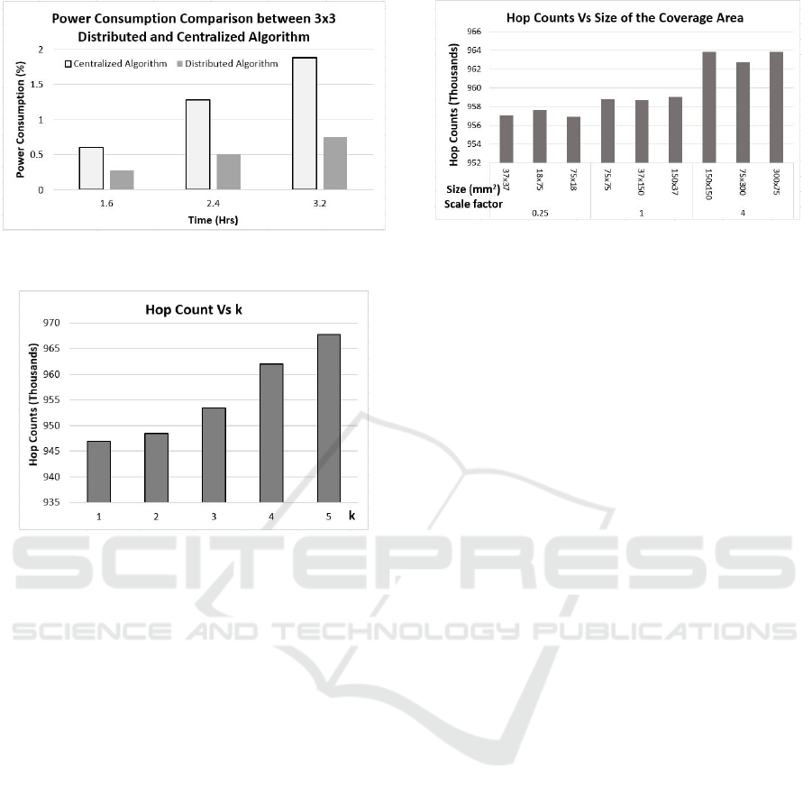
Figure 8: Average energy consumption comparison be-

tween distributed and centralized algorithm.

Figure 9: Performance k-MaxRS using different k values.

ber of resource-demanding principal sensors and the

relative decrease in the area of safe-regions for clus-

ters.

The effect of varying the size of WSN is illus-

trated in Figure 7. As expected, the rise in the num-

ber of nodes in WSN increases the hop count of both

the centralized and distributed algorithm. A notewor-

thy observation is that distributed technique (3 × 3)

performs better than the centralized scheme in all the

cases.

Figure 8 demonstrates an important feature of our

distributed scheme – overall less energy consumption,

which in turn increases overall network lifetime. We

ran both the distributed and centralized approach in

the default settings for 3.2 hours and computed aver-

age energy consumption over all the nodes in the net-

work. As can be seen in Figure 8, energy consump-

tion is at least 2-3 times more in centralized approach

than the distributed one. Also, as time increases, this

difference increases as well, indicating the efﬁcacy of

our proposed algorithm in the long run.

This experiment measured the number of hop

counts when the k values are varied at the end of the

second hour. Figure 9 shows that hop counts increase

for larger k since, when k is high, our algorithm needs

to send more possible solutions to the neighbor clus-

ters, resulting in more hop counts.

Figure 10: Performance k-MaxRS using different k values.

We did another experiment by changing the

shapes and sizes of the query region with the scale

factor of 4, and we measured the hop counts of differ-

ent query regions. Figure 10 measures the number of

hop counts once the shapes and size of the query re-

gion are changed – conﬁrming that the larger query

region is, more hop counts are needed. For larger

query region, each principle node has to transmit to

the neighbor clusters more data of the objects within

the area outside its cluster, extended by the size of

the speciﬁed query region. The larger extended area

would include more objects from other neighbor clus-

ters, and again each principle node has to send more

data/messages to other neighbor-clusters.

Our last experiments measured the variation of ac-

curacy of k-kMaxRS with the sampling rates (λ), re-

ported for two different sampling values: 1 and 5 min-

utes. We recorded the locations and weighted sums of

each MaxRS rectangle every minute, and compared

those outputs with the one where k-MaxRS is cal-

culated once every 5 minutes. We ran the experi-

ments for 10 times and averaged the percentage of

overlap of all k-MaxRSs – and we did the same for

the weights (measured in the optimally-located rect-

angles). The results, shown in Figure 11 illustrate that

the k-MaxRS at the lower sampling rate may induce

signiﬁcant errors in terms of keeping the sink up to

date – both in terms of the locations of R as well as

the values of the weighted sums. More speciﬁcally,

the results show the percentage of overlap of the val-

ues between the once-in-5 minutes sampling vs. sam-

pling every minute. The overlaps tend to reach 100%

by the end which, in a sense, is expected since the

phenomenon of interest is measured at t = 5 by both

setups. We note that the difference in energy con-

sumption was almost-linear – i.e., the sampling with

λ = 1 consumed approximately 5 times more energy

than the case of λ = 5. The investigation of balancing

the trade-off between the (im)precision and residual

energy (or overall lifetime) of the WSN, however, is

beyond the scope of this work.

Distributed In-Network Processing of k-MaxRS in Wireless Sensor Networks

115

5 RELATED WORKS

The MaxRS and its variants were ﬁrst tackled by

the researchers from computational geometry, de-

vising in-memory algorithms of O(n log n) time-

complexity (Imai and Asano, 1983; Nandy and Bhat-

tacharya, 1995). Motivated by applications from the

class of Location-Based Services (e.g., best location

for a new franchise store with a speciﬁed delivery

range; most attractive place for a tourist with a re-

stricted reachability), scalable solution for MaxRS in

spatial databases were proposed (Choi et al., 2012;

Choi et al., 2014). The distribution schemes proposed

in (Choi et al., 2014) work nicely for secondary mem-

ory settings but, it appears that the vertical subdivi-

sion of space used in those works is not well-suited

for WSN settings (cf. Section 3 and 4).

Recently, different variants of the MaxRS prob-

lem were investigated: – constraining locations of

the objects to an underlying spatial network (Phan

et al., 2014); – monitoring MaxRS over spatial

data streams (Amagata and Hara, 2016); – rotating-

MaxRS problem, i.e., allowing non axis-parallel rect-

angles (Chen et al., 2015). While interesting variants

of the traditional MaxRS problem, these works did

not consider the distributed processing aspects which

are typical for WSN settings, nor the multiple (k) so-

lutions.

A system implementing in-network solution to (a

single, k = 1) MaxRS query in WSN was presented

in (Hussain et al., 2015). We note that a similar phi-

losophy of hybrid hierarchical clustering and rout-

ing scheme (although tree-based, not digraph-based)

were used in (Avci et al., 014b), for different settings

– i.e., detecting and tracking evolving shapes in WSN.

Although there have been numerous works addressing

energy conservation in WSN (Anastasi et al., 2009),

to our knowledge, no energy-aware aggregation and

routing approaches exist for the k-MaxRS problem in

sensor networks.

Figure 11: Performance k-MaxRS processing using differ-

ent λ values.

6 SUMMARY & FUTURE

DIRECTION

We presented an efﬁcient distributed algorithm for

processing k-MaxRS queries in WSNs. The unique

nature of the k-MaxRS is that a collection of k ﬁxed-

size rectangles needs to be placed at distinct locations,

in a manner that ensures that the sum of the respective

(weighted) density/values in their interiors is maxi-

mized. We proposed a geographic clustering scheme

where principal nodes (i.e., cluster heads) not only

collect and aggregate data from their children, but

also communicate with the siblings (i.e., other prin-

cipals – predecessors and successors) in order to de-

tect the answer to the k-MaxRS query as early in the

hierarchy as possible, while reducing the overhead of

communicating with all the possible neighbors.

To the best of our knowledge, k-MaxRS has not

been addressed before in the context of WSNs and

there are multiple extensions and variants to be inves-

tigated, some of which we plan to address in the near

future. There are three distinct facets of the prob-

lem that we are currently focusing upon from com-

plementary perspectives: (1) The incorporation of the

(un)reliability of the links and transmission errors,

along with more detailed consideration of different

power-consumption models; (2) The investigation of

the impact of the discrepancy of the nodes locations

distribution; and (3) Dynamically adjusting the size

of the query-rectangle and/or k based on trade-offs

among different constraints (e.g., turnaround time,

overall energy consumption, “freshness” of the data

in the sink, etc.). In addition, we would like to inves-

tigate the incorporation of other kinds of dynamics-

related contexts: from the impact of the different

partitioning values (i.e., “m” and “n”) and adap-

tive congestion management (Ren et al., 2011; Wan

et al., 2003), through dynamic routing and aggrega-

tion structures (Fasolo et al., 2007), to incorporating

mobile nodes/sink (Mohamed et al., 2013).

ACKNOWLEDGMENTS

Research supported by NSF grants CNS-0910952 and

III 1213038, and ONR grant N00014-14-1-0215.

REFERENCES

Akyildiz, I. F., Su, W., Sankarasubramaniam, Y., and

Cayirci, E. (2002). Wireless sensor networks: A sur-

vey. Comput. Netw., 38(4):393–422.

SENSORNETS 2017 - 6th International Conference on Sensor Networks

116

Amagata, D. and Hara, T. (2016). Monitoring MaxRS in

spatial data streams. In EDBT, pages 317–328.

Anastasi, G., Conti, M., Di Francesco, M., and Passarella,

A. (2009). Energy conservation in wireless sensor net-

works: A survey. Ad hoc networks, 7(3):537–568.

Avci, B., Trajcevski, G., and Scheuermann, P. (2014b).

Managing evolving shapes in sensor networks. In

Proceedings of the 26th International Conference

on Scientiﬁc and Statistical Database Management,

page 22. ACM.

Bai, L. S., Dick, R. P., Chou, P. H., and Dinda, P. A.

(2011). Automated construction of fast and accurate

system-level models for wireless sensor networks. In

2011 Design, Automation & Test in Europe, pages 1–

6. IEEE.

Banerjee, I., Roy, I., Choudhury, A. R., Sharma, B. D.,

and Samanta, T. (2012). Shortest path based geo-

graphical routing algorithm in wireless sensor net-

work. In Communications, Devices and Intelligent

Systems (CODIS), 2012 International Conference on,

pages 262–265.

Chen, Z., Liu, Y., Wong, R. C.-W., Xiong, J., Cheng, X.,

and Chen, P. (2015). Rotating MaxRS queries. Infor-

mation Sciences, 305:110–129.

Choi, D.-W., Chung, C.-W., and Tao, Y. (2012). A scal-

able algorithm for Maximizing Range Sum in spa-

tial databases. Proceedings of the VLDB Endowment,

5(11):1088–1099.

Choi, D. W., Chung, C. W., and Tao, Y. (2014). Maxi-

mizing Range Sum in external memory. ACM Trans.

Database Syst., 39(3):21:1–21:44.

Fasolo, E., Rossi, M., Widmer, J., and Zorzi, M. (2007).

In-network aggregation techniques for wireless sensor

networks: A survey. Wireless Communications, IEEE,

14(2):70–87.

Ghica, O. C., Trajcevski, G., Scheuermann, P., Bischof, Z.,

and Valtchanov, N. (2008). Sidnet-swans: A simu-

lator and integrated development platform for sensor

networks applications. In Proceedings of the 6th ACM

Conference on Embedded Network Sensor Systems,

pages 385–386. ACM.

Hussain, M. M., Wongse-ammat, P., and Trajcevski, G.

(2015). Demo: Distributed MaxRS in wireless sensor

networks. In Proceedings of the 13th ACM Confer-

ence on Embedded Networked Sensor Systems, Sen-

Sys ’15, pages 479–480. ACM.

Imai, H. and Asano, T. (1983). Finding the connected

components and a maximum clique of an intersec-

tion graph of rectangles in the plane. Journal of al-

gorithms, 4(4):310–323.

Krishnamachari, B., Estrin, D., and Wicker, S. (2002).

The impact of data aggregation in wireless sensor

networks. In Distributed Computing Systems Work-

shops, 2002. Proceedings. 22nd International Confer-

ence on, pages 575–578. IEEE.

Li, H. and Tan, J. (2007). Heartbeat driven medium access

control for body sensor networks. In HealthNet, pages

25–30. ACM.

Madden, S. R., Franklin, M. J., Hellerstein, J. M., and

Hong, W. (2005). TinyDB: An acquisitional query

processing system for sensor networks. ACM Trans-

actions on database systems (TODS), 30(1):122–173.

Mohamed, M. M. A., Khokhar, A., and Trajcevski, G.

(2013). Energy efﬁcient in-network data indexing

for mobile wireless sensor networks. In Advances

in Spatial and Temporal Databases, pages 165–182.

Springer.

Nandy, S. C. and Bhattacharya, B. B. (1995). A uniﬁed

algorithm for ﬁnding maximum and minimum object

enclosing rectangles and cuboids. Computers & Math-

ematics with Applications, 29(8):45–61.

Phan, T.-K., Jung, H., and Kim, U.-M. (2014). An efﬁ-

cient algorithm for Maximizing Range Sum queries in

a road network. The Scientiﬁc World Journal, 2014.

Ren, F., He, T., Das, S. K., and Lin, C. (2011). Trafﬁc-

aware dynamic routing to alleviate congestion in wire-

less sensor networks. IEEE Trans. Parallel Distrib.

Syst., 22(9):1585–1599.

Trajcevski, G., Zhou, F., Tamassia, R., Avci, B., Scheuer-

mann, P., and Khokhar, A. (2011). Bypassing

holes in sensor networks: load-balance vs. latency.

In Global Telecommunications Conference (GLOBE-

COM 2011), 2011 IEEE, pages 1–5. IEEE.

Trigoni, N. and Krishnamachari, B. (2012). Sensor network

algorithms and applications. Philosophical Transac-

tions of the Royal Society of London A: Mathematical,

Physical and Engineering Sciences, 370(1958):5–10.

Wan, C.-Y., Eisenman, S. B., and Campbell, A. T. (2003).

CODA: Congestion detection and avoidance in sen-

sor networks. In Proceedings of the 1st international

conference on Embedded networked sensor systems,

pages 266–279. ACM.

Distributed In-Network Processing of k-MaxRS in Wireless Sensor Networks

117