
Virtualizing Closed-loop Sensor Networks: A Case Study
Priyanka Dattatri Kedalagudde and Michael Zink
Electrical and Computer Engineering, University of Massachusetts Amherst, Amherst, U.S.A.
Keywords:
Closed-loop Sensor Networks, Cyber-physical Systems, Virtualization.
Abstract:
Closed loop sensor networks are cyber-physical systems that establish a tightly coupled connection between
computational elements and the control of physical elements. Existing closed-loop sensor networks are based
on dedicated, ’stove-pipe’ architectures that prevent the sharing of these networks. This paper addresses the
problem of sharing these networks through virtualization. We propose scheduling algorithms that manage
requests from competing applications and evaluate their impact on system utilization as compared to a dedi-
cated network. These algorithms are evaluated through trace-driven simulations. We aim to demonstrate that
the proposed scheduling algorithms result in cost savings due to shared network infrastructure without unduly
affecting application utility. In our evaluations, we observe only a 20% reduction in average utility via the
DSES scheduling approach.
1 INTRODUCTION
Dynamic Data-Driven Application Systems
(DDDAS) (Allen et al., 2009; Brotzge et al.,
2004) are a new type of closed-loop sensor networks,
representing a sub-class of cyber-physical systems
(CPS) (Sztipanovits and Rajkumar, 2010). They have
the potential to save lives and property in the event
of natural disasters and also help increase national
security through critical infrastructure. Road-maps
for these sensor networks forecast the deployment of
thousands of actuable sensors (Council, 2008). These
networks differ from regular sensor networks in that
they perform actuated sensing, but also require a
control unit that determines future actuation.
Cost projections for the deployment and operation
of such infrastructures are in the order of billions of
dollars. These high costs are due to dedicated archi-
tectures and sensing resources that cannot be shared.
Sharing the physical substrate will significantly re-
duce the capital and operational costs while provid-
ing access to a broad set of applications that can run
on top of these infrastructures. To date, no instances
of such isolated, but fully shared closed-loop sensor
networks have been created. The fear of request in-
terference due to resource sharing, eventually leading
to data loss is a primary reason behind this adopter
apprehension.
Recent work (Drake et al., 2010) has demon-
strated that a network of radars such as CASA (Zink
et al., 2010; McLaughlin et al., 2009) has the poten-
Figure 1: Multi-application shared, closed-loop sensor net-
work.
tial of augment existing ones like NEXRAD and can
also be used to track low flying aircraft, making the
system well suited for sharing by weather and hard-
target tracking applications. Figure 1 illustrates this
operational capability.
This paper makes the following contributions:
• Architecture: We introduce an architecture for
virtualizing sensor networks and a design for a
virtualization layer. While the architecture also
includes networking and computational virtual-
ization, this paper focuses exclusively on the vir-
tualization layer.
• Scheduling: As a part of the virtualization layer,
we propose several scheduling approaches. In
contrast to traditional approaches used in com-
munication systems, our approaches utilize sen-
sor network specific characteristics like utility of
a sensing task and potential task overlap to make
scheduling decisions.
188
Dattatri Kedalagudde P. and Zink M.
Virtualizing Closed-loop Sensor Networks: A Case Study.
DOI: 10.5220/0006209901880195
In Proceedings of the 6th International Conference on Sensor Networks (SENSORNETS 2017), pages 188-195
ISBN: 421065/17
Copyright
c
2017 by SCITEPRESS – Science and Technology Publications, Lda. All rights reserved

The remainder of the paper is outlined as follows.
In Section 2, we present related work that has been
performed in the area of sensor network virtualiza-
tion. We formulate the problem statement in Sec-
tion 3. The overall architecture and design for the vir-
tualization layer is introduced in Section 4. Section 5
presents different scheduling approaches. We evalu-
ate these algorithms through trace-based simulations
as presented in Section 6. Concluding remarks and an
outlook on future work are given in Section 7.
2 RELATED WORK
Sensor network virtualization is not entirely a new re-
search area. Until now, the focus has been either on
the creation of virtual operating systems for sensor
nodes (Brouwers et al., 2009; Evensen and Meling,
2009; Hong et al., 2009) or the virtualization of net-
works that connect these nodes (Baumgartner et al.,
2010; Lim et al., 2009; Jayasumana et al., 2007).
Some approaches aim to abstract the sensor hardware
to simplify application development, but do not ad-
dress the sharing of resources, and are developed for
small sensor nodes (e.g., Atmel or Mica). Bose et
al. (Bose et al., 2007; Bose and Helal, 2008) were
the first ones to propose a service-oriented sensor net-
work architecture that is based on sensor virtualiza-
tion. In their approach, sensor virtualization is limited
to a virtual sensor abstracting a set of passive, physi-
cal sensors.
This concept has been extended by (Pumpichet
and Pissinou, 2010) for mobile sensors. Under a sim-
ilar concept proposed by Pajic and Mangharam, an
Embedded Virtual Machine (EVM) programming ab-
straction (Pajic and Mangharam, 2010) has been de-
veloped, that allows the composition of a virtual ma-
chine (VM) across physical nodes. In our work, VMs
do not span physical nodes but build a virtual slice
(as shown in Figure 2) across nodes. In the former
approach, a physical node can only be part of a sin-
gle VM making isolated sharing of the sensors be-
tween users impossible. Network sharing between
users/applications is one of the goals of our work.
The SATWARE (Massaguer et al., 2009) project
provides a middleware for sensor networks, and is
similar to our work, but it neither allows the isolated
sharing of sensors nor works on actuable sensors.
3 PROBLEM FORMULATION
Let us represent the sensor network as a set of sen-
sors S = s
1
,s
2
,s
3
,..,s
n
. A = a
1
,a
2
,a
3
,.., a
n
is a set of
applications that require access to sensors in S. X
s
i
(t)
is the system resource usage on a sensor s
i
∈ S at any
instant of time t . Utility is a measure of the quality
and applicability of the data generated by the sensor
for the application. The total utility U
s
i
and the total
system resources used X
s
i
for a specific application
a
i
∈ A on a sensor s
i
is given by:
Us
i
=
T
2
∑
t=T
1
Us
i
(t) (1)
Xs
i
=
T
2
∑
t=T
1
Xs
i
(t) (2)
where T
1
is the request start time and T
2
is the re-
quest termination time. U
s
i
(t) is the sensor’s utility at
a given instant. C(X
s
i
) is the cost of using a sensor’s
resources over a period of the application’s request.
On a dedicated sensor network, execution of an
application would result in a high level of utilization
for that application (
∑
n
i=1
U
s
i
), but at high infrastruc-
tural and operational costs.
Our goals are as follows:
• Reducing capital and operational costs by allow-
ing multiple applications to utilize a single, under-
lying sensor network, while maximizing system
utility simultaneously max(U
s
i
)∀a
i
∈ A.
• Minimizing the cost of using sensor resources,
min(C(X
s
i
))∀a
i
∈ A, thus potentially maximizing
revenue.
4 SYSTEM ARCHITECTURE
4.1 Overview
The following proposed architecture consists of three
major components in sensor network virtualization.
Figure 2 shows where these fit into the architecture.
• Sensor Virtualization Layer. This layer will en-
able multiplexing of different applications on a
unified substrate. This is achieved by developing
a class of scheduling algorithms that will schedule
and execute requests from different applications.
• Computation Virtualization Layer. We envi-
sion that users of sensor networks will be able to
obtain computational resources on-demand with-
out the need for owning dedicated resources from
compute clouds. Recent work has demonstrated
the feasibility of this approach for a short-term
weather forecast application that uses radar sensor
data (Krishnappa et al., 2012a; Krishnappa et al.,
2012b).
Virtualizing Closed-loop Sensor Networks: A Case Study
189

• Virtualization Toolkit. It is our goal to create
a virtualization toolkit that abstracts certain de-
tails of the sensor network from the application
developer to simplify development. Developers
should not have to deal with details such as ad-
mission control and task scheduling and the work
presented in this paper will create part of the un-
derlying foundation for this toolkit.
Figure 2: Closed-loop virtualized sensor network architec-
ture.
4.2 The Virtualization Layer
Virtualization is used to enable isolated applications
to share the use of computer hardware through virtual
machines (Seawright and MacKinnon, 1979; Barham
et al., 2003; Bugnion et al., 1997). Virtualizing
closed-loop sensor networks is a different challege
due to potential resource conflicts. For example, two
users might want to point their virtual radar to a differ-
ent azimuthal position at the same instant. Cognizant
of these constraints, we envision the architecture as
detailed below.
The Request Manager handles incoming requests
from the users and interfaces with the scheduler to
schedule them. The Scheduler then uses an algorithm
that takes into account sensor specific properties such
as utility and request overlaps to admit/deny different
tasks . The Data Manager is responsible for handing
the data back to the respective applications. This in-
cludes maintaining a mapping of merged/shared data
and their corresponding request IDs. When scan data
is generated, this componentresolves the request mul-
tiplexing and transfers the appropriate data based on
the mapping to the respective applications.
5 SCHEDULING APPROACHES
FOR THE VIRTUALIZATION
LAYER
5.1 TDMA Approaches
Here, we introduce a set of dynamic TDMA schedul-
ing approaches in which the time period T is fixed
but the slot length can be dynamic. Slot length is de-
fined as the request execution duration. We assume
that it takes 60 seconds to perform a scan (one heart-
beat). This can vary with each sensor installation, and
can be incorporated into our approach. We also as-
sume the time period T = 40s. This choice is dictated
by our use of CASA IP1 radar network’s data-set for
evaluation. The network always performs a low level
surveillance scan in the first 20 seconds of the heart-
beat and requested scans are executed in the remain-
ing 40 seconds.
We use the following equation as a base to calcu-
late the total utility for an application a
i
for a particu-
lar scheduling approach:
u(a
k
) =
n
∑
i=1
u
i
(a
k
hit
) −
n
∑
j=1
u
j
(a
k
miss
),i 6= j,∀a
k
∈ A,
where n represents the number of slots and
u
i
(a
k
hit
)/u
j
(a
k
miss
) are the application utilities if the re-
quested scan was executed/denied in that period re-
spectively.
Table 1: Sample data set for TDMA1 and TDMA2.
Slot Number Application Angle of scan Utility
9 B 30 1.3
10 B 30 1.7
10 C 120 1.8
11 A 180 1.3
11 C 120 1.8
11 B 30 1.7
12 A 180 1.3
13 C 120 1.8
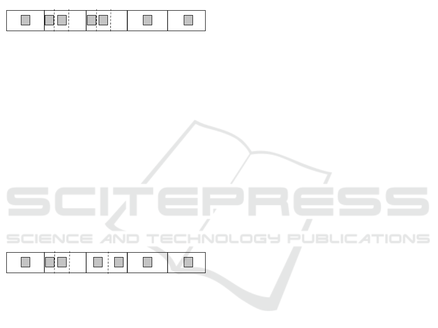
5.1.1 TDMA1 - Request Ratio Based Slot
Sharing
In this approach, the requested tasks in a heartbeat
are grouped based on the decreasing request ratio for
that slot. The request ratio is defined as number of
requests the application has made to the total number
of requests raised by all applications until that instant.
Application priority varies dynamically with the re-
quest ratio for each slot. This approach is useful in
scenarios where applications that require fresh infor-
mation continually need to be serviced first. For ex-
ample, in slot 11 of Table 1, the tasks A, B, and C
SENSORNETS 2017 - 6th International Conference on Sensor Networks
190
request sensor access at the same time. Subsequently,
requests B and C are scheduled since they have higher
request ratios than A (see Figure 3). The overall util-
ity for each application is:
u
A
TDMA1
= u
4
(A) − u
3
(A)
u
B
TDMA1
= u
1
(B) + u
2
(B) + u
3
(B)
u
C
TDMA1
= u
2
(C) + u
3
(C) + u
5
(C)
ACB CBB C
0
3T
2TT
4T 5T
A
10% 40%40%10%
Figure 3: Dynamic TDMA with decreasing request ratio
dependent slot sharing.
5.1.2 TDMA2 - Hit Ratio Based Slot Sharing
Here, the requested tasks are grouped based on the
increasing hit ratio of an application. The hit ratio
is defined as number of requests the application has
executed to the total number of requests raised by that
application until that instant. As previously, tasks A,
B and C in slot 11 have hit ratios that of 0, 1, and 1
respectively. Subsequently, A and C are scheduled for
execution within the given slot (see Figure 4).
u
A
TDMA2
= u
4
(A) + u
3
(A)
u
B
TDMA2
= u
1
(B) + u
2
(B) − u
3
(B)
u
C
TDMA2
= u
2
(C) + u
3
(C) + u
5
(C)
ACB CAB C
0
3T
2TT
4T 5T
A
60% 40%40%10%
Figure 4: Dynamic TDMA with increasing hit ratio depen-
dent slot sharing.
This approach tries to ensures that no application
is indefinitely starved of execution and balances fair-
ness by prioritizing applications based on their instan-
taneous hit ratios. This approach attempts to ensure
that application starvation does not occur in the pres-
ence of multiple, high priority applications.
5.2 Data Sharing Enabled Scheduling
(DSES)
In sensor networks, the data generated from one ap-
plication’s sensing activity can be of value to other
applications. For example, a thunderstorm sensing
application also measures rainfall, and the data from
these measurements can be utilized by a rainfall track-
ing application. While the former might scan the at-
mosphere at several elevations, the latter may require
scans only at the lowest elevation. Even though these
requests do not align perfectly, data generated by the
thunderstorm sensing’s lowest elevation scan is still
useful for the other application. We propose an algo-
rithm that attempts to multiplex applications by maxi-
mizing the data shared between overlapping requests.
5.2.1 The DSES Algorithm
This section details the data sharing algorithm of 1.
In an effort to build a tunable framework, we pro-
vide the user with two configurable parameters; a util-
ity threshold and an execution deadline. We evaluate
the feasibility of data sharing between requests using
these two parameters. The utility threshold is the ab-
solute minimum amount of data commonality (utility)
required for sharing to be considered feasible. The ex-
ecution deadline is the maximum time before which a
request has to finish executing. This is not a dura-
tion, but an absolute maximum bound on the execu-
tion time.
Some of the conventions used are as detailed here.
R1 is the request already executing on sensor s
1
at
time t
1
. R2 is the incoming request that also wants
sensor s
1
. (θ
s1,1
,θ
s1,2
) is the scan range of R1 and
(φ
s1,1
,φ
s1,2
) is for R2. t
exectime
is the execution time
for R1 and t
deadline
is the deadline for R2. R2
overlap
and R2
nonoverlap
represent the intersections of R1 and
R2’s scans, consequently determining Data
overlap
and
Data
nonoverlap
. In subsequent sections, we discuss the
different scenarios between competing requests.
5.2.2 Construction of Overlapping and
Non-overlapping Sets
Two competing requests R1 and R2 can be catego-
rized as non-overlapping, completely overlapping, or
partially overlapping based on their scan angles.
1. No Overlaps ((φ
s1,2
<= θ
s1,1
)∨(φ
s1,1
<= θ
s1,2
)):
If there is no overlap between the two requests R1
and R2, the execution of R2 is delayed, provided
the scheduler can guarantee that R2 can finish ex-
ecuting before its execution deadline. The request
is denied if this constraint cannot be met.
2. Complete Overlaps ((φ
s1,1
≥ θ
s1,1
) ∧ (φ
s1,2
≤
θ
s1,2
)): When the scan angle of the incoming re-
quest is a complete subset of an already executing
task for a given sensor, the data can be shared by
both requests. R1 receives all the data and R2 re-
ceives its share of data, up to 100%.
3. Partial Overlaps: If the incoming request is not a
complete subset of an executing request, the size
of the overlapping subset and its corresponding
utility is evaluated. Based on the scan angles of
Virtualizing Closed-loop Sensor Networks: A Case Study
191
the two requests, partial overlaps can have three
scenarios:
• Partial Overlap Scenario 1 ((φ
s1,1
< θ
s1,1
) ∧
(φ
s1,2
≤ θ
s1,2
) ∧ (φ
s1,2
> θ
s1,1
)): For example,
if (θ
s1,1
,θ
s1,2
) = (45
◦
,90
◦
) and (φ
s1,1
,φ
s1,2
) =
(0
◦
,90
◦
), then (45
◦
,90
◦
) represents the inter-
section of both requests and (0
◦
,45
◦
) represents
the non-overlapping set specific to R2.
• Partial Overlap Scenario 2 ((φ
s1,1
≥
θ
s1,1
) ∧ (φ
s1,2
> θ
s1,2
) ∧ (φ
s1,1
< θ
s1,2
)):
If (θ
s1,1
,θ
s1,2
) = (0
◦
,90
◦
) and (φ
s1,1
,φ
s1,2
) =
(45
◦
,135
◦
), then (45
◦
,90
◦
) represents the
intersection of R1 and R2, and (90
◦
,135
◦
)
represents the non overlapping set specific to
R2.
• Partial Overlap Scenario 3 ((φ
s1,1
< θ
s1,1
) ∧
(φ
s1,2
> θ
s1,2
)): If (θ
s1,1
,θ
s1,2
) = (45
◦
, 90
◦
)
and (φ
s1,1
,φ
s1,2
) = (0
◦
,135
◦
), then (0
◦
,45
◦
) and
(90
◦
,135
◦
) represents the non-overlapping set
specific to R2 and (45
◦
,90
◦
) represents the in-
tersection of both sets.
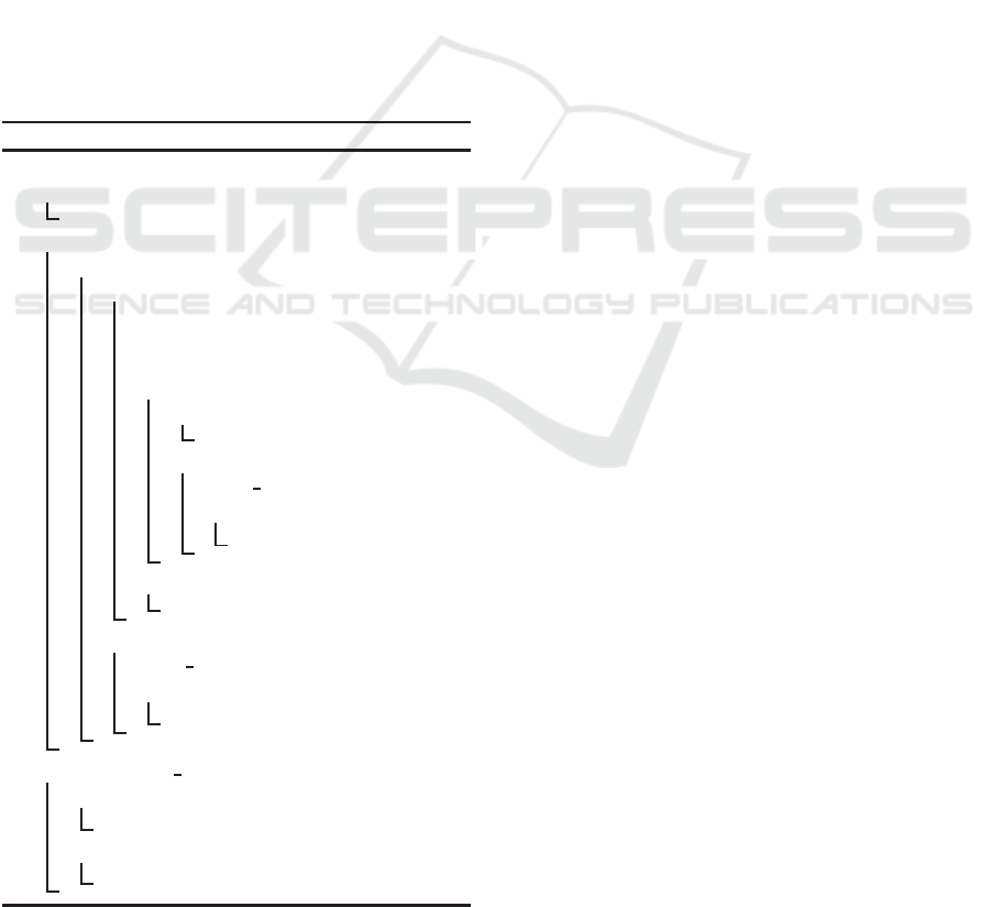
Algorithm 1: DSES Algorithm.
Sensor S
i
← Request R
if S
i
is idle then
Execute R
else
for task j in S
i
’s queue do
if R overlaps with j then
Data
overlap
← j
data
Data
nonoverlap
to S
i
’s queue
Calculate R
utility
if R
exectime
≤ R
deadline
then
if R
utility
≥ U
threshold
then
Execute R
else
delay task(R
delayed
)
if U
R
delayed
≥ U
threshold
then
Execute R
delayed
else
Cannot execute R
else
delay task(R
delayed
)
if U
R
delayed
≥ U
threshold
then
Execute R
delayed
Function delay task(R)
if R
delayed−exec
≤ R
deadline
then
Calculate R
utility
after delay
else
Cannot execute request R
Once the overlapping and non-overlapping sets
are constructed, the quantity of the overlapping data
that is useful for the incoming request is evaluated as
detailed in the following section.
5.2.3 Calculation of Percentage of Potential
Data Overlap
In this section, we present how the probable quantity
of the overlapping data Data
overlap
from the overlap-
ping requests is calculated if R1 and R2 possess a cer-
tain degree of overlap.
For example, if it takes 60 seconds to scan 360
◦
,
then it takes 1/6th of a second to scan 1
◦
. If R1 ar-
rives at time t
1
and R2 at time t
2
, then R1 would have
completed:
φ
′
s1,1
= θ
s1,1
+ (6 ∗ (t
2
− t
1
))
◦
when R2 arrives. The Data
overlap
equations for dif-
ferent cases of overlaps and non-overlaps are shown
in Table 2.
5.2.4 Effects on Non-overlapping Sets
In the absence of any overlap or for non-overlapping
sets, the execution of R2 is delayed as per Algo-
rithm 1. If the execution of R2 is delayed by n sec-
onds, the amount of data lost is:
φ
′
s1,1
= (θ
s1,1
+ (6 ∗ (n− t
2
))
◦
The Data
nonoverlap
equations for different cases of
overlaps and non-overlaps are shown in Table 2.
5.2.5 Calculation of Total Utility
The total utility for R2 is given by,
U = ((R2
overlap
∗ Data
overlap
) + (R2
nonoverlap
∗
Data
nonoverlap
))) ∗ (1− miss)
(3)
R2
overlap
∗ Data
overlap
is the quantity of data from the
overlapping set and R2
nonoverlap
∗ Data
nonoverlap
is the
quantity of data from the non-overlapping set. miss
represents whether a task has been scheduled (=0) or
1 otherwise. The total utility U for the cases of non-
overlap and overlaps are listed in Table 3.
6 EXPERIMENTAL EVALUATION
In this section, we present a series of results from sim-
ulations conducted on actual traces taken from a four
node radar sensor network (McLaughlin et al., 2009).
This network has different user groups (generally de-
scribed as applications in this paper) that request indi-
vidual tasks based on application preferences and the
past information generated by the radars.
SENSORNETS 2017 - 6th International Conference on Sensor Networks
192

Table 2: Data overlap in Overlapping and Non-Overlapping sets.
Type of Overlap Data
overlap
Data
nonoverlap
No Overlap 0 (θ
s1,1
− φ
′
s1,1
)/(θ
s1,1
− φ
s1,1
)
Complete Overlap ((φ
s1,2
− φ
′
s1,1
)/(φ
s1,2
− φ
s1,1
)) 0
Partial Overlap scenario 1 ((φ
s1,2
− φ
′
s1,1
)/(φ
s1,2
− θ
s1,1
)) (θ
s1,1
− φ
′
s1,1
)/(θ
s1,1
− φ
s1,1
)
Partial Overlap Scenario 2 ((θ
s1,2
− φ
′
s1,1
)/(θ
s1,2
− φ
s1,1
)) (φ
s1,2
− φ
′
s1,1
)/(φ
s1,2
− θ
s1,2
)
Partial Overlap Scenario 3 ((θ
s1,2
− φ
′
s1,1
)/(θ
s1,2
− θ
s1,1
)) ((θ
s1,1
− φ
′
s1,1
)/(θ
s1,1
− φ
s1,1
)) + ((φ
s1,2
− φ
′
s1,1
)/(φ
s1,2
− θ
s1,2
))
Table 3: Total Utility U for different cases of overlap.
Type of Overlap R2
overlap
R2
nonoverlap
Total Utility
No Overlap 0 1 (R2
nonoverlap
∗ Data
nonoverlap
) ∗ (1− miss)
Complete Overlap 1 0 (R2
overlap
∗ Data
overlap
) ∗ (1− miss)
Partial Overlap x%of(R2
overlap
+ R2
nonoverlap
) y%of(R2
overlap
+ R2
nonoverlap
) ((R2
overlap
∗ Data
overlap
) + (R2
nonoverlap
∗ Data
nonoverlap
)) ∗ (1 − miss)
We virtually schedule tasks according to the ap-
proaches presented in Section 5, calculate the utility
and then use this to compare the performance of dif-
ferent scheduling approaches.
6.1 Experimental Data Set
The dataset being used is generated from the CASA
system’s main control loop called Meteorological
Command and Control (MC&C) (Zink et al., 2009).
Saved features (meteorological features such as re-
flectivity) are fed into the simulator. There are five
different applications that generate tasks to scan dif-
ferent kinds of features at certain locations in the area
covered by the radars. To simulate a “stand-alone”
application on a dedicated sensor network, the sim-
ulator is run individually for each application gener-
ating a set of scan tasks. The scheduling algorithms
then operate on the combined set of tasks.
6.2 Results and Analysis
The reduction in utility of an application when com-
pared to its utility on a dedicated network is one of
the key performance indicators of efficiency. Any
scheduling mechanism that we consider will attempt
to minimize this utility reduction.
6.2.1 TDMA Approaches
Figure 5 plots the average utility against the ap-
plication’s request ratio for the various approaches.
TDMA2 is more consistent in the small sample space
of applications in maintaining an average reduction
in utility. Also, TDMA1 looks to perform in accor-
dance with the application request ratio, displaying
no reduction for high-request applications and a high
rate for rarely requested ones. We observe that aver-
age utility reduces for NWP even with a high request
rate. This is because NWP is mostly requested with
other applications that have higher request ratios and
longer execution times, thus preventing it from being
executed.
TDMA2 seems to be a better approach between
the two since it provides a fair distribution of re-
sources to all its applications and a tolerable reduc-
tion in utility. We evaluated the impact of utility for
the ’Res’ application and the average utility for this
application decreased by 30% when five applications
shared a sensor network.
Figure 5: Average Utility for TDMA approaches.
6.2.2 Data-sharing Based Approach
In our current design, the requests are either shared
(if they overlap) or are scheduled for execution later
if the scheduler can guarantee execution within the re-
quest’s deadline. From a service provider’s perspec-
tive, two requests that overlap completely mean opti-
mal cost of using system resources. The request that
began executing first obtains maximum utility. The
second that was piggybacked onto an executing one
receives a portion of the utility.
A request that has to be split into overlapping and
non-overlapping portions still results in lower cost
Virtualizing Closed-loop Sensor Networks: A Case Study
193
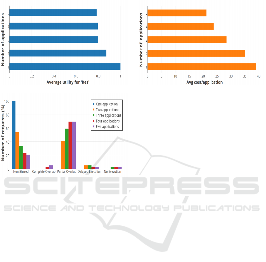
Figure 6: Average Utility per request in DSES.
Figure 7: Percentage of non-shared and shared tasks for
’Res’ application in DSES.
of resource usage because of the overlapping portion
that was shared with another request. The dedicated
resource usage needs to be taken into account only for
the non-overlapping portion.
Figure 6 illustrates a plot of average utility for ap-
plication ’Res’ with an increase in number of appli-
cations in the network. We see that the average util-
ity for ’Res’ decreases with an increase in number of
applications. Interestingly, the addition of a fifth ap-
plication causes the average utility of ’Res’ to slightly
decrease which may be attributed to a slight decrease
in unshared requests with the addition of the fifth ap-
plication. This is illustrated in Figure 7.
The average cost of using sensor resources to ex-
ecute a given request decreases with increase in num-
ber of applications. Figure 8 shows that the cost of re-
sources used per application starts to decrease as more
applications share the network. The average utility of
’Res’ decreases with an increase in number of appli-
cations, the impact due to request overlaps. The av-
erage utility for ’Res’ decreased by 20% as compared
to that on a dedicated network. From the results, we
see an improvement in the utility of application ’Res’
in DSES compared to TDMA.
Figure 8: Average cost of resource usage per application in
DSES.
7 CONCLUSIONS
In this paper, we introduced our architecture for
closed-loop sensor network virtualization. We be-
lieve that such an architecture can potentially reduce
the cost for creating and operating sensing infrastruc-
ture. Along with the architecture, we presented sensor
scheduling approaches and evaluated these through
trace-based simulations. Our results show that these
scheduling approaches allow the sharing of sensor
networks with a marginal reduction in overall utility.
Moving forward, we plan on developing a computa-
tional layer for sensor networks to provide an end-to-
end solution and plan to implement these scheduling
approaches in a two-node campus radar network.
ACKNOWLEDGEMENTS
This material is based upon work supported by the
National Science Foundation under Grant No. CNS-
1350752. Any opinions, findings, and conclusions
or recommendations expressed in this material are
those of the author(s) and do not necessarily reflect
the views of the National Science Foundation.
REFERENCES
Allen, G., Nabrzyski, J., Seidel, E., van Albada, G. D., Don-
garra, J. J., and Sloot, P. M. A., editors (2009). Com-
putational Science – ICCS 2009. Springer-Verlag.
Barham, P., Dragovic, B., Fraser, K., Hand, S., Harris, T.,
Ho, A., Neugebaue, R., Pratt, I., and Warfield, A.
(2003). Xen and the art of virtualization. In Pro-
ceedings of the 19th ACM Symposium on Operating
Systems Principles, Bolton Landing, NY, USA.
SENSORNETS 2017 - 6th International Conference on Sensor Networks
194

Baumgartner, T., Chatzigiannakis, I., Danckwardt, M.,
Koninis, C., Kr¨oller, A., Mylonas, G., Pfisterer, D.,
and Porter, B. (2010). Virtualising testbeds to support
large-scale reconfigurable experimental facilities. In
EWSN, pages 210–223.
Bose, R. and Helal, A. (2008). Distributed mechanisms for
enabling virtual sensors in service oriented intelligent
environments. In Intelligent Environments, 2008 IET
4th International Conference on, pages 1 –8.
Bose, R., Helal, A., Sivakumar, V., and Lim, S. (2007).
Virtual sensors for service oriented intelligent envi-
ronments. In Proceedings of the third conference on
IASTED International Conference: Advances in Com-
puter Science and Technology, ACST’07, pages 165–
170, Anaheim, CA, USA. ACTA Press.
Brotzge, J., Chandrasekar, V., Droegemeier, K., Kurose, J.,
McLaughlin, D., Philips, B., Preston, M., and Sekel-
sky, S. (2004). Distributed collaborative adaptive
sensing for hazardous weather detection, tracking, and
predicting. In Proceeding of Computational Science -
ICCS 2004, Krakow, Poland.
Brouwers, N., Langendoen, K., and Corke, P. (2009). Dar-
jeeling, a feature-rich vm for the resource poor. In
Proceedings of the 7th ACM Conference on Embedded
Networked Sensor Systems, SenSys ’09, pages 169–
182, New York, NY, USA. ACM.
Bugnion, E., Devine, S., and Rosenblum, M. (1997). Disco:
Running commodity operating systems on scalable
multiprocessors. ACM Transactions on Computer Sys-
tems, 15(4):143–156.
Council, N. R. (2008). Evaluation of the multifunction
phased array radar planning process. The National
Academic Press.
Drake, P., McLaughlin, D., and Nolan, M. (2010). Collab-
orative and adaptive sensing of the atmosphere (casa)
and multi-function sensor services network (mssn). In
Integrated Communications Navigation and Surveil-
lance Conference (ICNS), pages 1–33.
Evensen, P. and Meling, H. (2009). Sensor virtualiza-
tion with self-configuration and flexible interactions.
In Proceedings of the 3rd ACM International Work-
shop on Context-Awareness for Self-Managing Sys-
tems, Casemans ’09, pages 31–38, New York, NY,
USA. ACM.
Hong, K., Park, J., Kim, T., Kim, S., Kim, H., Ko, Y., Park,
J., Burgstaller, B., and Scholz, B. (2009). Tinyvm,
an efficient virtual machine infrastructure for sensor
networks. In Proceedings of the 7th ACM Conference
on Embedded Networked Sensor Systems, SenSys ’09,
pages 399–400, New York, NY, USA. ACM.
Jayasumana, A., Han, Q., and Illangasekare, T. (2007). Vir-
tual sensor networks - a resource efficient approach
for concurrent applications. In Proceedings of the 4th
International Conference on Information Technology:
New Generations (ITNG), Las Vegas, NV, USA.
Krishnappa, D. K., Irwin, D., Lyons, E., and Zink, M.
(2012a). Cloudcast: Cloud computing for short-term
mobile weather forecasts. In IPCCC 2012.
Krishnappa, D. K., Lyons, E., Irwin, D., and Zink, M.
(2012b). Network capabilities of cloud services for
a real time scientific application. In LCN 2012.
Lim, H. B., Iqbal, M., and Ng, T. J. (2009). A virtual-
ization framework for heterogeneous sensor network
platforms. In Proceedings of the 7th ACM Conference
on Embedded Networked Sensor Systems, SenSys ’09,
pages 319–320, New York, NY, USA. ACM.
Massaguer, D., Mehrotra, S., and Venkatasubramanian, N.
(2009). A semantic approach for building perva-
sive spaces. In Proceedings of the 6th Middleware
Doctoral Symposium, MDS ’09, pages 2:1–2:6, New
York, NY, USA. ACM.
McLaughlin, D., Pepyne, D., V.Chandrasekar, Philips, B.,
Kurose, J., and et al., M. Z. (2009). Short-Wavelenth
Technology and the Potential for Distributed Net-
works of Small Radar Systems. Bulletin of the Amer-
ican Meteorological Society (BAMS), 90(12):1797–
1817.
Pajic, M. and Mangharam, R. (2010). Embedded virtual
machines for robust wireless control and actuation.
In Real-Time and Embedded Technology and Applica-
tions Symposium (RTAS), 2010 16th IEEE, pages 79–
88.
Pumpichet, S. and Pissinou, N. (2010). Virtual sensor for
mobile sensor data cleaning. In GLOBECOM 2010,
2010 IEEE Global Telecommunications Conference,
pages 1 –5.
Seawright, L. and MacKinnon, R. (1979). Vm/370 - a study
of multiplicity and usefulness. IBM Systems Journal,
pages 4–17.
Sztipanovits, J. and Rajkumar, R., editors (2010). Interna-
tional Conference on Cyber-Physical Systems. ACM
Press.
Zink, M., Lyons, E., Westbrook, D., Kurose, J., and Pepyne,
D. (2010). Closed-loop architecture for distributed
collaborative adaptive sensing: Meteorogolical com-
mand & control. International Journal for Sensor Net-
works (IJSNET), 7(1/2).
Zink, M., Lyons, E., Westbrook, D., Pepyne, D., Pilips, B.,
Kurose, J., and Chandrasekar, V. (2009). Meteorog-
ical Command and Control: Architecture and perfor-
mance evaluation. In Geoscience and Remote Sensing
Symposium, 2008. IGARSS 2008. IEEE International.
Virtualizing Closed-loop Sensor Networks: A Case Study
195
