Strategic Capacity Expansion of a Multi-item Process with Technology

Mixture under Demand Uncertainty: An Aggregate Robust MILP

Approach

Jorge Weston, Pablo Escalona, Alejandro Angulo and Ra

ul Stegmaier

Deparment of Industrial Engineering, Universidad T

ecnica Federico Santa Mar

ıa, Valpara

ıso, Chile

Keywords:

Capacity Expansion, Machine Requirement Planning, Work Shifts, Robust Optimization.

Abstract:

This paper analyzes the optimal capacity expansion strategy in terms of machine requirement, labor force, and

work shifts when the demand is deterministic and uncertain in the planning horizon. The use of machines of

different technologies are considered in the capacity expansion strategy to satisfy the demand in each period.

Previous work that considered the work shift as a decision variable presented an intractable nonlinear mix-

integer problem. In this paper we reformulate the problem as a MILP and propose a robust approach when

demand is uncertain, arriving at a tractable formulation. Computational results show that our deterministic

model can ﬁnd the optimal solution in reasonable computational times, and for the uncertain model we obtain

good quality solutions within a maximum optimal gap of 10

−4

. For the tested instances, when the robust

model is applied with a conﬁdence level of 99%, the upper limit of the total cost is, on average, 1.5 times the

total cost of the deterministic model.

1 INTRODUCTION

When a manufacturing industry faces a scenario of

increasing demand in the long term and its facilities

are close to maximum capacity, the how to expand its

production capacity is a key decision. Strategic ca-

pacity expansion should determine the level of differ-

ent production factors over time, such as the number

of machines and workers needed to satisfy the pro-

duction requirement. The objective of this paper is

to determine the optimal capacity expansion strategy

that minimizes the machinery investment cost, the la-

bor cost, the production cost, and the idle capacity

cost over a deﬁned planning horizon, when the future

demand is uncertain and there is no knowledge of its

distribution. The decision variables are (i) the pro-

duction requirements needed to satisfy the demand

in each period, (ii) the number of machines of each

technology needed, (iii) the work shifts necessary to

cover the production requirement, and (iv) the work-

ers needed to perform the number of shifts. This con-

siders simultaneously the machine requirement plan-

ning (MRP) and the strategic capacity planning under

uncertainty.

In this paper, we developed a multi-item, and

multi-period model with technology mixture that de-

termines the optimal expansion strategy considering

the machine numbers of each technology, labor, and

work shifts needed to satisfy the demand. We consid-

ered two different cases: when the demand is deter-

ministic and when it is uncertain. For the ﬁrst case, we

formulated a mixed integer linear program (MILP),

which can be solved efﬁciently with a mixed-integer

solver. Then, we incorporated the demand uncertainty

into the deterministic model, following a robust ap-

proach that considers the best worst case and a non-

anticipativity constraint. In this formulation, ﬂexi-

bility is provided to the model via a box-type uncer-

tainty set obtaining a robust model with adjustable ro-

bustness; the non-anticipativity constraints, to make

the problem tractable, are represented by afﬁne de-

cision rules. The model with demand uncertainty is

also an MILP and can be solved with a mixed-integer

solver. We used both models to evaluate the impact of

a technology mixture in the capacity expansion strat-

egy. We considered three types of technology that dif-

fer in terms of production rate, worker requirements,

investment cost and production cost.

The main contributions of this work are: (i) An

efﬁcient formulation of a strategic capacity expansion

model that considers the work shifts as a decision

variable; and (ii) the inclusion of the uncertain nature

of the demand in the model under a robust approach.

The rest of this paper is structured as follows. In

Section 2, a brief literature review is presented, and

then, in Section 3 we present the model formulation

for the two cases, when the demand is deterministic

and when the demand is uncertain. In Section 4, we

Weston J., Escalona P., Angulo A. and Stegmaier R.

Strategic Capacity Expansion of a Multi-item Process with Technology Mixture under Demand Uncertainty: An Aggregate Robust MILP Approach.

DOI: 10.5220/0006202201810191

In Proceedings of the 6th International Conference on Operations Research and Enterprise Systems (ICORES 2017), pages 181-191

ISBN: 978-989-758-218-9

181

report our computational results, and ﬁnally, in Sec-

tion 5 we conclude and present future extensions to

this work.

2 RELATED WORK

A strategic capacity expansion problem consists of

deﬁning the expansion sizes and expansion timing in

order to meet the incremental demands within a long-

term planning horizon. The objective is to minimize

the total costs with respect to the expansion process

(Luss, 1982). On the other hand, machine require-

ment planning (MRP) can be deﬁned as the speciﬁ-

cation of the number of each type of machine needed

in each period for a productive process (Miller and

Davis, 1977).

A comprehensive review of the strategic capac-

ity expansion problem can be found in Luss (1982),

Van Mieghem (2003), Wu et al. (2005), Julka et al.

(2007), and Geng et al. (2009) and a more recent

review in Mart

ınez-Costa et al. (2014). In particu-

lar, Mart

ınez-Costa et al. (2014) described the major

decisions and conditioning factors involved in strate-

gic capacity planning. They classiﬁed the strategic

capacity expansion models according to the number

of sites involved in the expansion process (a single

or multiple sites), the type of the capacity expansion

considered (expansion by investing/purchasing, out-

sourcing/subcontracting, reduction and replacement),

whether the uncertainty of the parameters is consid-

ered in the problem formulation, and ﬁnally, the type

of mathematical programming model and its solution

procedure.

Our model corresponds to a single-site and multi-

item capacity expansion problem under uncertain de-

mand. We consider that capacity expansion can be

achieved through machine acquisition and / or by us-

ing a ﬂexible workforce in terms of increasing or de-

creasing the number of shifts. In this sense, the tra-

ditional structure of the strategic capacity expansion

problem does not consider the relationship between

the workforce planning and capacity acquisition de-

cisions. This is related to the natural separation be-

tween strategic and tactical decision making. How-

ever, when these decisions are addressed separately,

sub-optimal solutions are frequently the result. Since

workforce ﬂexibility and capacity acquisition can rep-

resent substitutable magnitudes, ﬂexible workforce

options could be also considered as a means of in-

creasing capacity. In particular, for capital intensive

companies, the implementation of one or more shift is

an additional tool that managers can use to increment

capacity continuously, avoiding the huge investment

cost related to equipment acquisition.

To the best of our knowledge, only Fleischmann

et al. (2006), Bihlmaier et al. (2009), and Escalona

and Ram

ırez (2012) considered the workforce in their

strategic capacity planning. Fleischmann et al. (2006)

studied a multi-site and multi-item strategic capac-

ity model with machine replacement and overtime as

a means to meeting demand. They considered the

same average cost for any overtime, such as prolonga-

tion of a shift, weekend shifts, night shifts, or regular

third shifts. The model is formulated as an MILP and

solved directly using CPLEX. Bihlmaier et al. (2009)

analyzed a multi-site and multi-item strategic capac-

ity model without machine replacement that inte-

grates tactical workforce planning via shift work im-

plementation. They consider a detailed set of shifts,

such as a late shift, night shift, Saturday shift, and Sat-

urday late shift. They presented a two-stage stochas-

tic MILP for strategic capacity planning under uncer-

tain demand that is solved by Benders decomposition.

Escalona and Ram

ırez (2012) studied the optimal ex-

pansion strategy of a process, in terms of machinery,

labor, and work shifts, through an aggregated model

without machine replacement. They considered that

in the process one, two, or three shifts can be worked

per time period. The main difﬁculty related to their

model is that shifts are not linear with the number of

machines and workers needed to meet the demand.

The model is formulated as a mixed integer nonlin-

ear problem and solved by complete enumeration by

ﬁxing the shifts during the planning horizon.

Our strategic capacity model also considers un-

certain demand. Four primary approaches to consid-

ering uncertainty exist (Sahinidis, 2004), which ba-

sically comprise (i) stochastic programming, where

the uncertain parameters are considered random vari-

ables with known probability distributions; (ii) fuzzy

programming, where some variables are considered

as fuzzy numbers; (iii) stochastic dynamic program-

ming, where random variables are combined with dy-

namic programming; and (iv) robust optimization,

where the uncertainty of the parameters do not follow

a known probability distribution, and the solutions are

robust, i.e., they perform best in the worst case.

In the literature, two-stage stochastic program-

ming is a dominant approach to handling stochas-

tic capacity planning under various uncertainties

(Swaminathan, 2000), (Hood et al., 2003), (Barahona

et al., 2005), (Christie and Wu, 2002), (Karabuk and

Wu, 2003), (Geng et al., 2009), (Rastogi et al., 2011),

(Levis and Papageorgiou, 2004), and (Bihlmaier et al.,

2009). A major shortcoming of two-stage stochastic

programming is that it generates only a static capac-

ity expansion plan and neglects the dynamic adjust-

ICORES 2017 - 6th International Conference on Operations Research and Enterprise Systems

182

ments based on new information when the demand is

revealed in each period. Several studies have adapted

stochastic dynamic programming to overcome this is-

sue (Rajagopalan et al., 1998), (Asl and Ulsoy, 2003),

(Cheng et al., 2004), (Li et al., 2009), (Stephan et al.,

2010), (Wu and Chuang, 2010), (Pratikakis et al.,

2010), (Chien et al., 2012), (Pimentel et al., 2013),

and (Lin et al., 2014).

In summary, few previous research studies on

strategic capacity planning considered the workforce

as a tool for increasing or decreasing capacity, and to

the best of our knowledge, no robust optimization ap-

proach exists for dealing with demand uncertainty in

strategic capacity planning.

3 MODEL FORMULATION

Consider a capacity expansion problem of a process

over a planning horizon of T (t = 1, ..., τ) periods. In

this process, I (i = 1, ..., n) items are produced, and

J ( j = 1, ..., m) technologies are available for their

production. The demand for item i in the period t

is d

. Without loss of generality, we assume that the

aggregate demand (

∑

i∈I

) will increase on the long

term, i.e., the aggregate demand follows a positive

trend.

Let r

i j

be the production rate of item i produced

with technology type j, and let ¯µ

be the maximum

utilization for each machine of type j that will be con-

sidered by the design requirement. In each period it is

possible to work K shifts (k = 1, 2, 3); in each shift the

available working time is limited by H

. The number

of shifts that will be worked in the period t is deter-

mined by the binary variable W

, which will be 1 if

k shifts are used in period t, else it will be 0. The

number of machines of type j needed in each shift to

satisfy the demand in period t working k turns is de-

noted by Y

jkt

; the number of machines of type j that

will be acquired in period t is denoted by V

; and the

number of machines available at the beginning of the

planning horizon (t = 0) is B

To meet the demand in each period of the planning

horizon, the capacity expansion could happen by: (i)

acquiring new machines (expansion by investment) or

(ii) modifying the number of shifts (expansion by op-

erational cost). Therefore, in each period it is possi-

ble to hire or ﬁre workers. Let Uh

be the number

of workers hired at the beginning of the period t to

operate machines of type j, and let U f

be the num-

ber of workers ﬁred at the beginning of the period t

that operated machines of type j. The workers avail-

able to operate machines of type j in the period t is

denoted by O

, with O

= A

representing the work-

ers available at t = 0. The number of workers needed

to operate one machine of technology type j is repre-

sented by

. Finally, the quantity of item i produced

with technology type j in each period t is represented

by the variable X

i jt

For this problem the costs that will be considered

are: (i) the investment cost of acquiring a machine

of type j in the period t (CI

); (ii) the unitary labor

cost in period t (CL

); (iii) the production cost for one

item i produced in a machine of type j in the period

t (Cp

i jt

); (iv) the opportunity cost incurred by idle

capacity of technology type j (Cop

); and, ﬁnally,

(v) the unitary cost of hiring and ﬁring, denoted by

and C

respectively. It will be assumed that all

the mentioned costs are properly brought to present

value. A glossary of the terms used in the following

sections can be found in appendix A. For this work we

are going to consider the cost of opening or closing a

shift as negligible, even if in reality they are not cost-

free.

3.1 Deterministic Formulation

When demand is deterministic we propose the follow-

ing capacity expansion problem, denoted by (P0).

Problem (P0):

min

X,V,Y,Uh,Uf,W

TC =

(

∑

i jt

∑

Cop

∑

l=1..t

−

∑

jkt

∑

k Y

jkt

∑

U f

)

(1)

s.t:

∑

j∈J

i jt

≥ d

∀i,t (2)

∑

i∈I

i jt

≤ ¯µ

∑

k∈K

k Y

jkt

∀ j, t (3)

∑

k∈K

jkt

≤ B

∑

l=1..t

∀ j, t (4)

∑

k∈K

= 1 ∀t (5)

jtk

≤ M W

∀ j, t, k (6)

∑

k∈K



jkt

−Y

j,k,t−1



−U f

∀ j, t (7)

∑

k∈K



jk0



∀ j (8)

X ≥ 0 (9)

Strategic Capacity Expansion of a Multi-item Process with Technology Mixture under Demand Uncertainty: An Aggregate Robust MILP

Approach

183

Y, Uh, Uf, V ∈ Z

(10)

W ∈

{

0, 1

}

(11)

The objective is to minimize the total cost (TC), con-

sidering the production cost, opportunity cost, invest-

ment cost, labor cost, and the cost of ﬁring or hiring

workers. The satisfaction of demand is ensured by

(2). Constraint (3) restricts the total demanded time

by the total available time; (4) ensures that the num-

ber of machines of technology j available in the pe-

riod t is greater than the number of machines needed

to satisfy the demand assigned in that period to the

technology j. Constraints (5) and (6) ensure that the

number of work shifts used in period t are of only one

type, i.e., k = 1 or k = 2 or k = 3. Constraint (7) rep-

resents the continuity and requirement for workers in

each period t, and constraint (8) represents an initial

condition.

It is easy to show that the problem (P0) is equiv-

alent to the problem presented by Escalona and

Ram

ırez (2012) by incorporating the constraints (4)

and (5) and considering the following equivalences of

variables:

∑

k∈K

jkt

(12)

= ND

− ND

j,t−1

(13)

= B

∑

l=1..t

(14)

∑

k∈K

jkt

(15)

where w

is the decision variable that determines the

number of shifts needed in period t, NN

is the num-

ber of machines of type j needed in the period t to

satisfy the demand, and ND

is the number of ma-

chines of type j available in the period t.

3.2 Uncertain Formulation

In this paper we use a robust approach, where the un-

certainty set is deﬁned as a box, which is a partic-

ular case of the polyhedral set (Bertsimas and Sim,

2004),(Bertsimas and Thiele, 2006), (Guigues, 2009),

and the problem is formulated as an afﬁne multi-stage

robust model with a simpliﬁed afﬁne policy (Lorca

et al., 2016).

Given the uncertain nature of the demand, it can-

not be predicted with exactitude. In the best scenario,

the estimate of the demand will be close to the ac-

tual value, but this will not happen frequently. The

most frequent outcome is to have a variation (delta)

between the estimate and actual demand. This delta

tends to increase as the period analyzed is further in

the future. When the variation is positive, the com-

pany over-produces, incurring a cost for not selling

the excessive units produced; this cost can be esti-

mated using the production cost or an opportunity

cost. On the other hand, if this delta is negative, the

demand cannot be completely satisﬁed; in this case

the cost incurred by the company is one of lost sales.

The lost-sale cost is often discussed since it can result

in a loss of proﬁt, a loss of future clients, or the loss of

clients whose demand could not be satisﬁed, causing

a bad reputation and loss of conﬁdence in the com-

pany. Taking this into consideration, a negative delta

is highly undesirable, and therefore it is fundamen-

tal to determine how to address the uncertain nature

of the demand such that this delta is non-negative (or

even 0) most of the time.

Let D



| d

∈



− Γ

+ Γ



the uncertainty set of d

, where

is the nominal

value of the demand, and let Γ represent the conserva-

tiveness of the model that can be associated with the

risk factor of the companies. Denote by D the aggre-

gate uncertainty set, i.e., D = ∪

Since we sought a robust model that can avoid

a negative delta, our worst case will be the one that

consider the maximum value that d

can take under

the uncertainty set D

; in this case this corresponds

+ Γ

. Therefore, the demand satisfaction con-

straint for the robust model can be written as

∑

j∈J

i jt

≥

+ Γ

∀i,t (16)

Replacing (2) in the problem (P0) by (16), we

obtain a robust model denoted by (P1). It is easily

noticed that the deterministic problem has two dif-

ferent types of decision variables: (i) strategic de-

cisions, i.e., decisions that affect the productivity in

the long term and cannot be modiﬁed at the moment

of demand realization; and (ii) operational decisions

that are made in each period and which therefore de-

pend on the realization of the demand. In the second

type we have the production quantity decision vari-

able (X). This variable has a clear dependence on

the demand realization, dependence that will be ad-

dressed via an afﬁne decision rule of the form

X(d)

i jt

+ λ

i j

∑

τ=1



iτ

−

iτ



, (17)

where the ﬁrst term (

i jt

) represents the nominal value

of the quantity of item i to be produced in period t

with machines of type j, and λ

i j

is the percentage of

the accumulated over-demand assigned to the item i

and machines of technology j. Taking the deﬁnition

of the uncertain set (D) and the afﬁne decision rules

deﬁned by (17) and incorporating them in problem

(P0), we obtain our afﬁne multi-stage robust model

denoted by (P2).

ICORES 2017 - 6th International Conference on Operations Research and Enterprise Systems

184

Problem (P2):

min

χ,V,Y,Uh,Uf,W,λ,Z

(

Z +

∑

Cop

∑

l=1..t

−

∑

jkt

∑

k Y

jkt

∑

U f

)

(18)

s.t: (4), (5), (6), (7), (8), (9), (10), (11)

∑

j∈J

i jt

+ λ

i j

∑

τ=1



iτ

−

iτ



≥ d

∀i,t,d (19)

∑

i∈I

i jt

+ λ

i j

∑

τ=1



iτ

−

iτ



¯µ

i jt

≤

∑

k∈K

k Y

jkt

∀ j, t, d (20)

∑

i jt

+ λ

i j

∑

k=1



−



i jt

≤ Z ∀d (21)

∑

i j

= 1 (22)

Z ∈ ℜ

, λ ∈ [0, 1] (23)

We created the auxiliary variable Z in constraint

(21) to denote the worst-case production cost. Con-

straints (19) and (20) are obtained by replacing the

variable X in constraints (2) and (3) by the afﬁne de-

cision rule (17).

Making some straightforward arrangements, and

taking into consideration that constraints (19)-(21)

are robust constraints that should hold for all d ∈ D,

which is equivalent to maximizing each constraint

over the uncertainty set D, it is possible to replace

constraints (19)–(21) with the following set of con-

straints:

∑

i jt

≥ Γ

1 −

∑

i j

∑

i j

t−1

∑

τ=1

iτ

∀i,t

(24)

∑

i jt

∑

i j

i jt

∑

τ=1

iτ

≤ ¯µ

∑

k∈K

k Y

jkt

∀ j, t

(25)

∑

i jt

∑

k=t

∑

i jk

i j

≤ Z (26)

With these replacements, we obtained a MILP that

considers the uncertain nature of the demand and that

can be solved by a MIP solver in reasonable compu-

tational time. Note that if Γ

= 0, the solution is equal

to the problem (P0) (the nominal problem).

4 COMPUTATIONAL STUDY

The computational study was developed with the fol-

lowing objectives: (i) evaluate the computational per-

formance (in terms of CPU time) of the proposed

model compared with that presented in the literature;

(ii) analyze the behavior of the total cost to changes of

Γ, i.e., analyze how the total cost grows as more de-

mand (over its expected value) is considered; and (iii)

test the applicability of our model in an industrial-size

example. Since problems (P0) and (P1) are particular

cases of (P2), we will only analyze (P2).

All experiments were performed with an AMD A6

2.0 GHz processor with 6 GB RAM memory, and the

models were solved using CPLEX 12.6.

4.1 Industrial Size Example

We implemented our model using the information

presented by a cosmetic company about a packaging

process, in particular a sachet ﬁlling one, of four items

that have high growth potential in the long term. For

this process, three types of technology were evalu-

ated. These technologies differ in (i) investment cost,

(ii) unitary production cost, and (iii) workers required

to operated one machine. For this implementation, we

considered a time horizon of ten periods with each pe-

riod being one year.

The cosmetic company provided the demand fore-

cast for each item, i.e., the nominal value of the de-

mand and the standard deviation of the forecast er-

ror. For each item and each period, the company

treated the uncertainty through reliability intervals of

the form

± σ

1−

, where

is the demand fore-

cast for the item i at period t, Z

1−

is the quantile

associated with a conﬁdence level of 1 − α, and σ

corresponds to the standard deviation of the forecast

error for item i at period t. Note that for this reliability

interval, the company assumed that the forecast errors

are Gaussian white noise.

Treating the demand uncertainty via re-

liability intervals can be easily related to

the demand uncertainty set deﬁned in Sec-

tion 3.2 through the following relationships

, Γ = Z

1−

, and

= σ

, ∀i ∈ I, t ∈ T .

Therefore, the demand uncertainty set to be

used in this illustrative example is of the form

| d

∈

− Z

1−

+ Z

1−

where Z

1−

∈ {0, 0.25, 0.52, 0.84, 1.28, 1.64,

1.96, 2.33, 2.58, 3.29}, which corresponds to

conﬁdence levels of 0%, 20%, 40%, 60%, 80%,

90%, 95%, 98%, 99%, and 99.9%, respectively.

Each problem has 343 variables (133 continuous,

Strategic Capacity Expansion of a Multi-item Process with Technology Mixture under Demand Uncertainty: An Aggregate Robust MILP

Approach

185

180 integer, and 30 binary variables) and 235 linear

constraints.

For this computational study we considered the

following set of parameters:

• Demand: The nominal value of demand and the

standard deviation of the forecast error are pre-

sented in Table 2 and Table 3 in B.

• Production rate (r

i j

): The production rate is the

same for each type of technology, i.e., r

i j

, ∀ j ∈ J, r

= 120, r

= 170, r

= 400, and

= 600.

• Maximum utilization (µ

): µ

= 0.8, µ

= 0.9,

= 0.98.

• Available time per shift (H

): 2080[hours].

• Number of workers needed per machine of tech-

nology j (

= 3,

= 2, and

= 1.

• Investment cost (CI

): CI

= CI

(1.15)

1−t

, ∀t =

{2, ..., T }, with CI

1,1

= $25000, CI

2,1

= $50000,

and CI

3,1

= $75000.

• Opportunity cost (Cop

): Cop

= CI

f , ∀ j ∈

J, ∀t ∈ T , where f represents the relation between

the useful life and the depreciation time of the ma-

chine, and corresponds to 0.10.

• Annual labor cost per worker (CL

= CL

(1.15)

1−t

, ∀t = {2, ..., T }, with

= $16032.

• Unitary production cost (C p

i jt

): The produc-

tion cost will depend only on the type of

technology, i.e., Cp

i jt

= Cp

, ∀i ∈ I, Cp

(1.15)

1−t

, ∀ j ∈ J, ∀t = {2, ..., T }, with

1,1

= $1, C p

2,1

= $0.75, and C p

3,1

= $0.5.

• Unitary ﬁring and hiring cost: C

= $500 and

= $4500.

• Initial conditions: The number of workers and

machines available at the beginning of the plan-

ning horizon, for each technology, are 0, i.e.,

= A

= 0, ∀ j ∈ J.

4.2 Results of the Industrial Size

Example

The expansion route for this problem involves differ-

ent shifts and the use of only one type of technol-

ogy. According to the results, the technology type se-

lected is, regardless of the value of α, the one with the

highest investment cost but with the lowest produc-

tion cost and fewest required workers (type 3). The

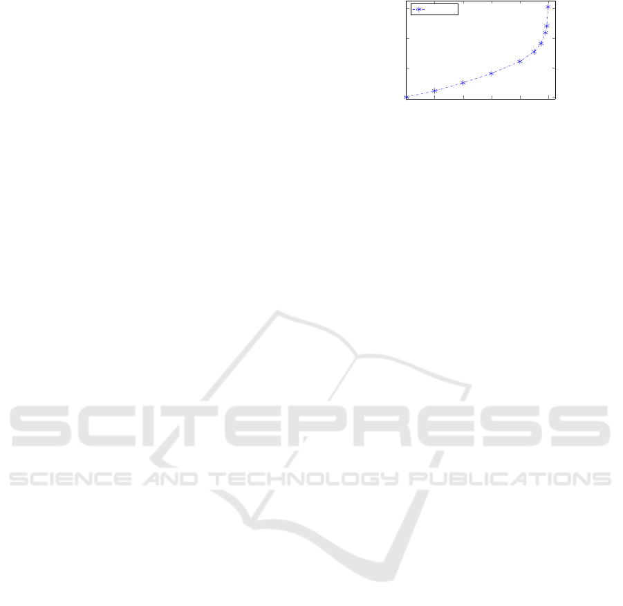
nominal total cost for the expansion under determin-

istic demand (1 − α = 0) is $8152716. In Figure 1 we

0 0.2 0.4

0.6

0.8 1

1.2

1.4

1.6

1 −α

Total Cost

Figure 1: Total cost behavior.

show the proportion of the total cost over the nominal

cost for each value of 1− α.

From Figure 1 we observe that the total cost in-

creases exponentially when more variable demand is

considered, and therefore each percentage increase is

more expensive than the previous one; for example, if

a reliability level (1−α) of 0.9 is selected, i.e., the de-

mand can be satisﬁed 95% of the time, the total cost

increases to 1.3 times the nominal cost, but if the reli-

ability level selected is 0.99 ,the total cost increases to

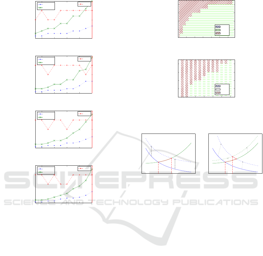
1.48 times the nominal cost. Figure 2 presents the ex-

pansion route in terms of shifts, total number of ma-

chines, and total number of workers needed in each

period for four different instances. In all instances,

we observed that the shifts changed along the plan-

ning horizon, and that an operational expansion (in-

creasing the number of shifts) is always preferred be-

fore realizing an investment; with this is possible to

determine that is more advisable to expand via shifts

before purchasing more machines. Therefore, if the

shifts are considered ﬁxed, it is possible to arrive at

sub-optimal solutions.

4.3 Sensitivity Analysis

To analyze the impact of the parameters in the ex-

pansion strategy, we developed a sensitivity analy-

sis, where the following parameters were varied: (i)

investment cost, (ii) operational cost, and (iii) num-

ber of workers. For each one the technology mixture

and the shifts structure will be analyzed considering a

conﬁdence level of 0.9, i.e., Γ = Z

0.95

= 1.64. The

shifts structure will be considered as the aggregate

number of shifts along the planning horizon (ANS),

i.e., ANS=

∑

t,k

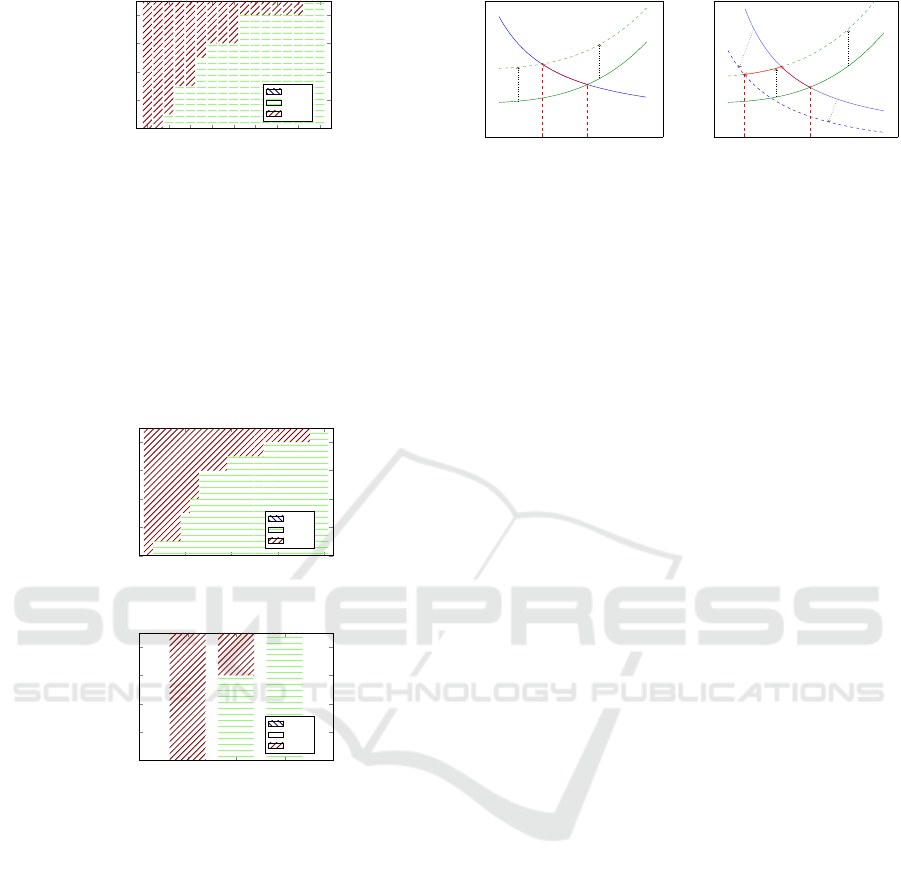
Investment Cost. The investment cost of the actual

selected technology type ( j = 3) was increased until it

is not selected anymore. This increase was measured

with respect to technology type 1. Figure 3 shows

the technology mixture versus the investment cost of

technology type 3, (a) when the operational costs are

different for each type of technology and (b) when

they are the same.

From Figure 3 is possible to observe a gradual

transference from machines of technology type 3 to

ICORES 2017 - 6th International Conference on Operations Research and Enterprise Systems

186

2 4

8 10

Time Period

Workers - Machines

Machines

Workers

2 4

8 10

Shifts

(a) 1 − α = 0 (Γ = 0)

2 4

8 10

Time Period

Workers - Machines

Machines

Workers

2 4

8 10

Shifts

(b) 1 − α = 0.8 (Γ = 1.28)

2 4

8 10

Time Period

Workers - Machines

Machines

Workers

2 4

8 10

Shifts

2 4

8 10

Time Period

Workers - Machines

Machines

Workers

2 4

8 10

Shifts

(d) 1 − α = 0.999 (Γ = 3.29)

Figure 2: Expansion route by Γ.

machines of technology type 2. Note that this trans-

ference happens sooner when the operational costs are

the same for all the technologies. In particular, from

Figure 3(a), total transference is achieved when the

investment cost of technology type 3 is at least 131

times CI

, and from Figure 3(b), total transference is

achieved when the investment cost of the machines of

type 3 is 14 times the investment cost of machines of

type 1.

We observe that the ANS increases when the in-

vestment cost increases. This behavior can be ex-

plained for two cases, when the rise of the invest-

ment cost (i) does not induce technology mixture, and

(ii) when it does induce technology mixture. Figure

4 shows the behavior of the cost equilibrium under

varying investment cost for both cases.

When the increase in the investment cost does not

induce technology mixture (Figure 4(a)), the aggre-

gate investment cost curve moves upwards and the

aggregate labor cost stays unchanged. This implies

0 20 40

80 100 120

Times CI

Number of machines

Type 1

Type 2

Type 3

(a) Different operational cost

(C p

i1t

> C p

i2t

> C p

i3t

)

2 4

8 10 12 14

Times CI

Number of machines

Type 1

Type 2

Type 3

(b) Same operational cost

(C p

i jt

= C p

∀ j ∈ J)

Figure 3: Sensitivity to investment cost.

ANS

(a) Without technology

mixture

ANS

(b) Under technology mix-

ture

Figure 4: Equilibrium dynamic under investment cost vari-

ation.

that the equilibrium moves from point A to point A

resulting in a higher cost and a higher ANS. In the

second case, when the increase in the investment cost

induces technology mixture (Figure 4(b)), the curve

dynamic can be explained in two stages: (i) the aggre-

gate investment cost increases and (ii) the aggregate

labor cost also simultaneously increases; with this the

equilibrium moves from point B to point C and ﬁnally

to point B

. Note that, since in this case the aggregate

investment cost increases signiﬁcantly more than the

labor cost, the new equilibrium achieved at point B

implies a higher cost and a higher ANS.

Operational Cost. The operational cost of the actual

selected technology ( j = 3) was increased until the

model stopped selecting it. This increase was mea-

sured with respect to technology type 1. Figure 5

shows the technology mixture under varying produc-

tion cost.

From Figure 5, it is possible to observe a gradual

transference from machines of technology type 3 to

machines of technology type 2. When the operational

cost of the machines of type 3 is 1.19 times that of ma-

chines of type 2, the technology transference is total.

Strategic Capacity Expansion of a Multi-item Process with Technology Mixture under Demand Uncertainty: An Aggregate Robust MILP

Approach

187

0.74

0.76

0.78 0.8 0.82 0.84

0.86

0.88 0.9

Times C p

i1t

Number of machines

Type 1

Type 2

Type 3

Figure 5: Sensitivity to operational cost.

We also observed that without technology mixture the

ANS does not change.

Number of Workers. Similar to the previous anal-

ysis the number of workers required for technology

type 3 was increased until the technology transfer-

ence was total. The resulting technology mixture is

presented in Figure 6, (a) when the operational costs

are different for each type of technology and (b) when

they are the same.

Number of workers needed (

)

Number of machines

Type 1

Type 2

Type 3

(a) Different operational cost

(C p

i1t

> C p

i2t

> C p

i3t

)

1 2 3

Number of workers needed (

)

Number of machines

Type 1

Type 2

Type 3

(b) Same operational cost

(C p

i jt

= C p

∀ j ∈ J)

Figure 6: Sensitivity to required number of workers.

From Figure 6 it is possible to observe a grad-

ual transference from machines of technology type

3 to machines of technology type 2. Note that this

transference starts when both technologies require the

same number of workers, and is more drastic when

the operational cost is the same for all the technolo-

gies (Figure 6(b)).

In this analysis is also possible to note a relation-

ship between the number of workers and the ANS. An

increase in the number of workers implies a decrease

in the ANS. Two cases can be recognized: when the

rise in the number of workers (i) does not induce tech-

nology mixture, and (ii) when it does induce technol-

ogy mixture. Figure 4 shows the behavior of the cost

equilibrium under a variation of the workers require-

ment for both cases.

ANS

(a) Without technology

mixture

ANS

(b) Under technology mix-

ture

Figure 7: Equilibrium dynamic under variation in the re-

quired number of workers.

When the increase in the number of workers does

not induce technology mixture (Figure 7(a)), the ag-

gregate labor cost curve moves upwards and the ag-

gregate investment cost stays unchanged. This im-

plies that the equilibrium moves from point D to point

, resulting in a higher cost with a lower ANS. In

the second case, when the increase in the number

of workers induces technology mixture (Figure 7(b)),

the curve dynamic can be explained in two stages: (i)

the aggregate labor cost increases and (ii) the aggre-

gate investment cost simultaneously decreases; with

this the equilibrium moves from point E to point F

and ﬁnally to point E

. Note that the aggregate la-

bor cost varies signiﬁcantly more than the investment

cost and the new equilibrium is achieved at point E

implying a higher cost and a lower ANS.

For this industrial-size example, on average, 90%

of the cost can be explained as operational. Therefore,

when the operational costs are the same for all types

of technology, the technology mixture is more sen-

sitive under variation of the investment cost or num-

ber of workers. From the sensitivity analysis, we ob-

served that (i) the optimal capacity expansion strategy

is more sensitive to the cost that has more inﬂuence

over the total cost, (ii) the required number of work-

ers is always an important decision factor even when

the labor cost represents less than 10% of the total

cost, and (iii) the ANS has a direct relationship with

the investment cost and an inverse one with the labor

cost.

4.4 Computational Performance

To evaluate the computational performance of our

model and to cover a wide range of data, we generated

a set of 180 problems, each one randomly generated

around a base case with 10 different items, 5 types of

technologies, and a planning horizon of 10 periods,

with each problem having 881 variables (551 contin-

uous, 300 integer, and 30 binary variables) and 412

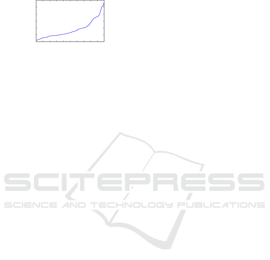
linear constraints. Figure 8 shows the computation

times in log

(sec) for all instances. In the abscissa

the cumulative percentage of instances is presented.

ICORES 2017 - 6th International Conference on Operations Research and Enterprise Systems

188

0.1 0.2 0.3 0.4

0.5 0.6

0.7 0.8 0.9 1

−2

Cumulative percentage

Time [log

(sec)]

Figure 8: Computation Times.

Figure 8 shows that we observed reasonable com-

putation times; 80% of the instances were solved in

less than 10 seconds and 94% of the instances were

solved in less than 100 seconds, with a geometric

mean of 2.8 seconds. The nominal problem of this

instances where solved with the formulation and algo-

rithm presented in Escalona and Ram

ırez (2012) ob-

taining an average computational of 584585 seconds

to arrive at the optimal solution, therefore our formu-

lation has an average speedup of 25175x.

5 CONCLUSION

In this paper, we develop a capacity expansion model

for multi-product, multi-machine manufacturing sys-

tems with uncertain demand. At ﬁrst, a linear deter-

ministic model is presented and later the demand un-

certainty is incorporated using a robust approach for-

mulating an afﬁne multi-stage robust model. In con-

trast with most of the works presented in the literature,

our model considers the shifts as a decision variable,

allowing more ﬂexibility in the type of expansion that

can be used.

For instances that consider a planning horizon of

10 periods, 10 items, and with 5 types of technologies

available, the computation times prove to be reason-

able ones with times below 100 seconds for most of

them (94%), and therefore our model performs bet-

ter than the one presented in the literature, having an

average speedup of 25175x.

From the instances that we tested, we observed the

following managerial insights:

• Fixing beforehand the number of shifts to work

along the planning horizon can take us to sub-

optimal solutions.

• The technology mixture is most sensitive to the re-

quired number of workers and to the most impor-

tant cost.

• There exists an inverse relationship between la-

bor cost (number of workers) and the aggregate

available time and a direct relationship between

investment cost and the aggregate available time.

• The operational cost by itself does not change

the aggregate available time; in fact, if there is

no change in the investment cost and number of

workers, then the aggregate available time does

not change, i.e. the available time, and there-

fore the work shifts routed along that planning

horizon, depend only on the investment and labor

costs.

An interesting discussion that escaped the scope

of this work is the analysis of some costs, such as the

cost incurred when opening or closing a shift and the

opportunity cost which can be determined following

business logic instead of the accounting logic used in

this work.

Possible extensions of this problem that can be

considered are (i) the use of a scenario approach

with multi-stage programming (Ben-Tal et al., 2009),

(Shapiro, 2009), (ii) the use of CVaR

∆

to minimize

the variability of the solution (Rockafellar and Urya-

sev, 2000), (Pﬂug, 2000), (Rockafellar et al., 2006)

instead of cost minimization, and (iii) considering un-

certainty of other parameters such as the maintenance

times, production rates, costs, and/or available times.

REFERENCES

Asl, F. M. and Ulsoy, A. G. (2003). Stochastic optimal

capacity management in reconﬁgurable manufactur-

ing systems. CIRP Annals-Manufacturing Technol-

ogy, 52(1):371–374.

Barahona, F., Bermon, S., Gunluk, O., and Hood, S. (2005).

Robust capacity planning in semiconductor manufac-

turing. Naval Research Logistics, 52(5):459–468.

Ben-Tal, A., El Ghaoui, L., and Nemirovski, A. (2009). Ro-

bust optimization. Princeton University Press.

Bertsimas, D. and Sim, M. (2004). The price of robustness.

Operations research, 52(1):35–53.

Bertsimas, D. and Thiele, A. (2006). Robust and data-

driven optimization: Modern decision-making under

uncertainty. INFORMS Tutorials in Operations Re-

search: Models, Methods, and Applications for Inno-

vative Decision Making.

Bihlmaier, R., Koberstein, A., and Obst, R. (2009). Model-

ing and optimizing of strategic and tactical production

planning in the automotive industry under uncertainty.

OR spectrum, 31(2):311–336.

Cheng, L., Subrahmanian, E., and Westerberg, A. W.

(2004). Multi-objective decisions on capacity plan-

ning and production-inventory control under uncer-

tainty. Industrial & engineering chemistry research,

43(9):2192–2208.

Chien, C.-F., Wu, C.-H., and Chiang, Y.-S. (2012). Co-

ordinated capacity migration and expansion planning

for semiconductor manufacturing under demand un-

certainties. International Journal of Production Eco-

nomics, 135(2):860–869.

Strategic Capacity Expansion of a Multi-item Process with Technology Mixture under Demand Uncertainty: An Aggregate Robust MILP

Approach

189

Christie, R. M. and Wu, S. D. (2002). Semiconductor capac-

ity planning: stochastic modelingand computational

studies. IIE Transactions, 34(2):131–143.

Escalona, P. and Ram

ırez, D. (2012). Expansi

on de capaci-

dad para un proceso, m

ultiples

ıtems y mezcla de tec-

nolog

ıas. In 41 Jornadas Argentinas de Informatica.

Fleischmann, B., Ferber, S., and Henrich, P. (2006). Strate-

gic planning of bmw’s global production network. In-

terfaces, 36(3):194–208.

Geng, N., Jiang, Z., and Chen, F. (2009). Stochastic pro-

gramming based capacity planning for semiconductor

wafer fab with uncertain demand and capacity. Euro-

pean Journal of Operational Research, 198(3):899–

908.

Guigues, V. (2009). Robust production management. Opti-

mization and Engineering, 10(4):505–532.

Hood, S. J., Bermon, S., and Barahona, F. (2003). Capacity

planning under demand uncertainty for semiconductor

manufacturing. Semiconductor Manufacturing, IEEE

Transactions on, 16(2):273–280.

Julka, N., Baines, T., Tjahjono, B., Lendermann, P., and Vi-

tanov, V. (2007). A review of multi-factor capacity

expansion models for manufacturing plants: Search-

ing for a holistic decision aid. International Journal

of Production Economics, 106(2):607–621.

Karabuk, S. and Wu, S. D. (2003). Coordinating strategic

capacity planning in the semiconductor industry. Op-

erations Research, 51(6):839–849.

Levis, A. A. and Papageorgiou, L. G. (2004). A hierarchical

solution approach for multi-site capacity planning un-

der uncertainty in the pharmaceutical industry. Com-

puters & Chemical Engineering, 28(5):707–725.

Li, C., Liu, F., Cao, H., and Wang, Q. (2009). A

stochastic dynamic programming based model for un-

certain production planning of re-manufacturing sys-

tem. International Journal of Production Research,

47(13):3657–3668.

Lin, J. T., Chen, T.-L., and Chu, H.-C. (2014). A stochastic

dynamic programming approach for multi-site capac-

ity planning in tft-lcd manufacturing under demand

uncertainty. International Journal of Production Eco-

nomics, 148:21–36.

Lorca, A., Sun, X. A., Litvinov, E., and Zheng, T.

(2016). Multistage adaptive robust optimization for

the unit commitment problem. Operations Research,

64(1):32–51.

Luss, H. (1982). Operations research and capacity ex-

pansion problems: A survey. Operations research,

30(5):907–947.

Mart

ınez-Costa, C., Mas-Machuca, M., Benedito, E., and

Corominas, A. (2014). A review of mathematical pro-

gramming models for strategic capacity planning in

manufacturing. International Journal of Production

Economics, 153:66–85.

Miller, D. M. and Davis, R. P. (1977). The machine require-

ments problem. The International Journal of Produc-

tion Research, 15(2):219–231.

Pﬂug, G. C. (2000). Some remarks on the value-at-risk

and the conditional value-at-risk. In Probabilistic con-

strained optimization, pages 272–281. Springer.

Pimentel, B. S., Mateus, G. R., and Almeida, F. A. (2013).

Stochastic capacity planning and dynamic network

design. International Journal of Production Eco-

nomics, 145(1):139–149.

Pratikakis, N. E., Realff, M. J., and Lee, J. H. (2010). Strate-

gic capacity decision-making in a stochastic man-

ufacturing environment using real-time approximate

dynamic programming. Naval Research Logistics

(NRL), 57(3):211–224.

Rajagopalan, S., Singh, M. R., and Morton, T. E. (1998).

Capacity expansion and replacement in growing

markets with uncertain technological breakthroughs.

Management Science, 44(1):12–30.

Rastogi, A. P., Fowler, J. W., Carlyle, W. M., Araz, O. M.,

Maltz, A., and B

uke, B. (2011). Supply network

capacity planning for semiconductor manufacturing

with uncertain demand and correlation in demand

considerations. International Journal of Production

Economics, 134(2):322–332.

Rockafellar, R. T. and Uryasev, S. (2000). Optimization of

conditional value-at-risk. Journal of risk, 2:21–42.

Rockafellar, R. T., Uryasev, S., and Zabarankin, M. (2006).

Optimality conditions in portfolio analysis with gen-

eral deviation measures. Mathematical Programming,

108(2-3):515–540.

Sahinidis, N. V. (2004). Optimization under uncertainty:

state-of-the-art and opportunities. Computers &

Chemical Engineering, 28(6):971–983.

Shapiro, A. (2009). On a time consistency concept in risk

averse multistage stochastic programming. Opera-

tions Research Letters, 37(3):143–147.

Stephan, H. A., Gschwind, T., and Minner, S. (2010). Man-

ufacturing capacity planning and the value of multi-

stage stochastic programming under markovian de-

mand. Flexible services and manufacturing journal,

22(3-4):143–162.

Swaminathan, J. M. (2000). Tool capacity planning for

semiconductor fabrication facilities under demand un-

certainty. European Journal of Operational Research,

120(3):545–558.

Van Mieghem, J. A. (2003). Commissioned paper: Capacity

management, investment, and hedging: Review and

recent developments. Manufacturing & Service Oper-

ations Management, 5(4):269–302.

Wu, C.-H. and Chuang, Y.-T. (2010). An innovative ap-

proach for strategic capacity portfolio planning under

uncertainties. European Journal of Operational Re-

search, 207(2):1002–1013.

Wu, S. D., Erkoc, M., and Karabuk, S. (2005). Managing

capacity in the high-tech industry: A review of litera-

ture. The Engineering Economist, 50(2):125–158.

ICORES 2017 - 6th International Conference on Operations Research and Enterprise Systems

190

APPENDIX

A Glossary of Terms

Table 1: Glossary of terms.

Sets Deﬁnition

I Set of items indexed by i

J Set of type of machines indexed by j

T Set of periods indexed by t

K Set of number of shifts indexed by k, with k = 1,2, 3

Parameters

i jt

Unitary production cost for item i produced with a machine of type j in period t

Investment cost of a machine of type j in period t

Cop

Opportunity cost for a machine of type j in period t

Unitary labor cost in period t

Hiring cost

Firing cost

Number of machines of type j available at the beginning of the planning horizon

Number of workers available to operate the machines of type j at the beginning of the planning horizon

Demand realization of item i in period t

Nominal demand of item i in period t

Maximum perturbation for the demand of item i in period t

i jt

Production rate of items i with machine of type j in period t

¯µ

Maximum utilization of machines type j

Available working time for each work shift

M A big enough number

Number of workers needed to operate one machine of type j

Γ Level of conservativeness of the model

Demand forecast of the item i at period t

Standard deviation of the forecast error for item i at period t

Variables

i jt

Number of items i produced with machines of type j in period t

Number of machines of type j bought in period t

jkt

Number of machines of type j needed in each shift to satisfy the demand in period t, working k shifts

1 if k shifts are worked in period t, 0 otherwise

Number of workers hired in period t to work machines of type j

U f

Number of workers ﬁred in period t that worked machines of type j

Number of shifts to work in the period t

Number of machines of type j needed at period t to satisfy the demand

Number of machines of type j available at period t

i j

Percentage of the accumulated over-demand assigned to the item i and machine j

i jt

Nominal quantity of item i to be produced in period t with machines of type j

Z Worst case production cost.

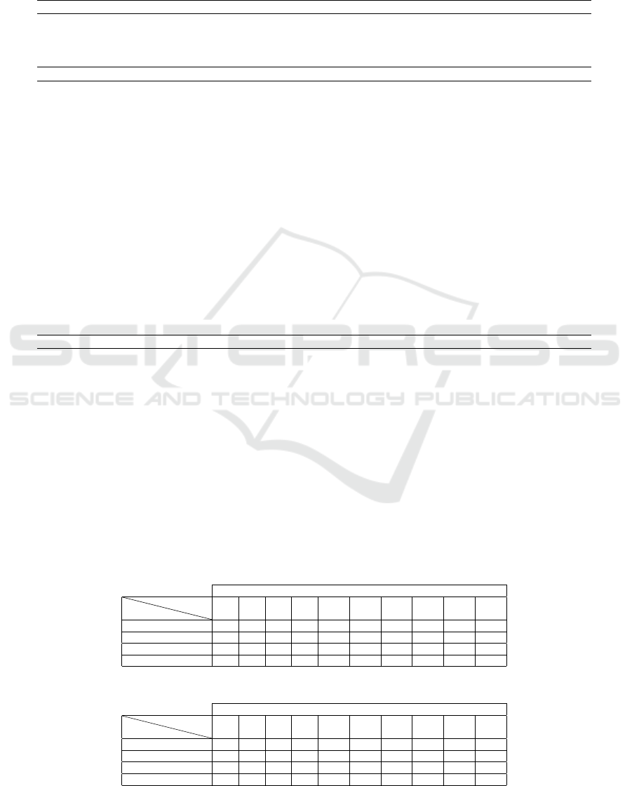
B Data for Illustrative Example

Table 2: Demand forecast of the item i at period t.

[∗10

units]

1 2 3 4 5 6 7 8 9 10

1 100 111 122 138 177 236 330 411 483 605

2 328 420 549 662 788 950 1091 1479 1651 1830

3 367 470 650 762 1021 1140 1293 1736 2227 3111

4 180 226 308 391 523 686 942 1089 1452 1815

Table 3: Standard deviation of the forecast error for item i at period t.

[∗10

]

1 2 3 4 5 6 7 8 9 10

1 30 44 53 70 99 179 292 416 515 858

2 83 130 210 343 532 823 1051 1771 2740 3823

3 142 243 468 747 1126 1335 1829 2590 4040 7805

4 67 96 155 236 423 742 1232 1685 3088 5054

Strategic Capacity Expansion of a Multi-item Process with Technology Mixture under Demand Uncertainty: An Aggregate Robust MILP

Approach

191