Exact Approach to the Scheduling of F-shaped Tasks with Two and

Three Criticality Levels

Antonin Novak

1,2

, Premysl Sucha

and Zdenek Hanzalek

1,2

Czech Institute of Informatics, Robotics and Cybernetics, Czech Technical University in Prague, Prague, Czech Republic

Department of Control Engineering, Faculty of Electrical Engineering, Czech Technical University in Prague,

Prague, Czech Republic

Keywords:

Scheduling, Mixed-criticality, Embedded Systems, Integer Linear Programming.

Abstract:

The communication is an essential part of a fault tolerant and dependable system. Safety-critical systems are

often implemented as time-triggered environments, where the network nodes are synchronized by clocks and

follow a static schedule to ensure determinism and easy certiﬁcation. The reliability of a communication bus

can be further improved when the message retransmission is permitted to deal with lost messages. However,

constructing static schedules for non-preemptive messages that account for retransmissions while preserving

the efﬁcient use of resources poses a challenging problem. In this paper, we show that the problem can be

modeled using so-called F-shaped tasks. We propose efﬁcient exact algorithms solving the non-preemptive

message scheduling problem with retransmissions. Furthermore, we show a new complexity result, and we

present computational experiments for instances with up to 200 messages.

1 INTRODUCTION

The communication buses in modern vehicles are an

essential part of advanced driver assistants. Those

systems depend on the data gather by sensors, such as

LIDAR, cameras, and radars. The data describing the

surrounding environment are communicated through

communication buses to ECUs (Electronic Control

Units) where they are processed, and appropriate ac-

tions are taken. For example, if an obstacle is detected

in front of the vehicle, the car automatically activates

breaks. Not only driver assistant systems rely on the

communication. Different ECUs are responsible for

running the car as a whole. The fuel is injected ac-

cordingly to the current combustion and outside con-

ditions and cars with the drive-by-wire system steer

via electronic signals.

The modern vehicle is considered as a fault-

tolerant and dependable system. If one part of it

breaks down or does not work as expected, the hu-

man life is in risk. Since the intra-vehicular com-

munication is the key element of the car, it is sub-

ject to a safety certiﬁcation. The safety certiﬁcation

is a process, where the manufacturer proves that his

safety-critical systems such as autonomous driving

are working correctly to a high degree of assurance.

If manufacturers are not able to demonstrate the cor-

rect behavior of the central communication bus, then

the whole certiﬁcation process is not complete. Ac-

cording to SSR Automotive Warranty & Recall Report

2016, the number of software-related recalls in 2015

accounted for 15% of all recalls, marking the impor-

tance of the certiﬁcation.

Traditionally, event-triggered communication pro-

tocols are commonly used in automotive industry. In

the event-triggered environment, the actions are per-

formed on-demand, i.e. triggered by some events.

Even though, event-triggered protocols are ﬂexible,

their usage in modern cars is limited due to certiﬁca-

tion and veriﬁcation issues. The response time analy-

sis (i.e. the analysis of the behavior of the system) in

real-life event-triggered communication systems in-

cluding gateways and precedence relations is a very

complex problem, therefore the safety certiﬁcation of

systems utilizing the event-triggered environment is a

difﬁcult task (Baruah and Fohler, 2011).

An alternative to event-triggered real-time sys-

tems is the time-triggered paradigm. Messages

in time-triggered communication are transferred

through the network at speciﬁc times prescribed by

a static pre-computed static schedule. The sched-

ule is constructed usually with tools known from

OR/Mathematical Optimization ﬁeld (Dvorak and

Hanzalek, 2016; Kopetz et al., 2005) such that it re-

160

Novak A., Sucha P. and Hanzalek Z.

Exact Approach to the Scheduling of F-shaped Tasks with Two and Three Criticality Levels.

DOI: 10.5220/0006198101600170

In Proceedings of the 6th International Conference on Operations Research and Enterprise Systems (ICORES 2017), pages 160-170

ISBN: 978-989-758-218-9

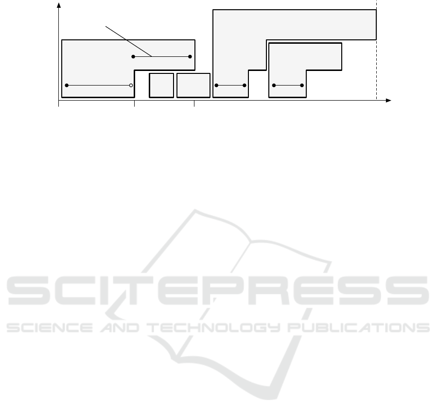
criticality levelcriticality level

timetime

max

execution scenari oexecution scenari o

Figure 1: A feasible schedule of F-shaped tasks with a runtime execution scenario denoted by the black line.

spects the problem and safety constraints. Therefore,

the certiﬁcation of the system is achieved via showing

feasibility of the produced communication schedule.

The determinism and veriﬁability of time-

triggered communications led to the design of proto-

cols that includes time-triggered communication for

safety-critical systems. For example, FlexRay bus

is used nowadays in the automotive industry (e.g.

Porsche Panamera, Nissan Inﬁnity Q50). One of the

disadvantages of time-triggered protocols is their non-

ﬂexibility. For example, the static schedule does not

take into consideration the message retransmission.

The retransmission occurs when a highly critical mes-

sage is not delivered e.g. due to EM noise. A possi-

ble solution how to enable message retransmissions in

static time-triggered schedules is to allocate more pro-

cessing time for each message to account for possible

retransmissions. If no retransmission occurs during

an actual execution, then the resource is idle until the

start time of the next message. However, since re-

transmissions do not appear as frequently, the average

resource utilization would be poor.

In this paper, we introduce a new solution to this

problem. We build static schedules that allow retrans-

mission of non-preemptive messages to some degree.

An extra time needed for retransmissions is compen-

sated by skipping less critical messages. The trick

we use to solve the problem is to include a part of

the problem solution to its formulation. Instead of

scheduling rectangles, denoting the single exact pro-

cessing time of a message, we schedule so-called F-

shapes. This leads to an interesting combinatorial

problem, where we are given a set of shapes that

are aligned on the left side with the right side that is

jagged (see an example in Fig. 1). The goal is to pack

these shapes as tightly as possible so that they do not

overlap.

The use of F-shapes is a very elegant solution that

achieves efﬁcient resource utilization. It modiﬁes the

traditional scheduling problem into the challenging

one where the schedule has to assume alternatives

based on the observed runtime scenario. Even though

there is an exponential number of possible runtime

scenarios, and for each of them, the static schedule

is well-deﬁned, we will show, that the introduced for-

malism makes the problem computationally tractable

in practice.

1.1 Application to Automotive

Frequently, in the complex systems, functionalities

with different criticality co-exist on a single bus. The

adaptation of IEC 61508 safety standard (Bell, 2006),

the ASIL, deﬁnes the application levels with a haz-

ard assessment corresponding to three Safety Integrity

Levels. Therefore the schedules with three criticality

levels arise from the application in the automotive do-

main:

• messages with high criticality (criticality level 3)

are used for safety-related functionalities (their

failure may result in death or serious injury to peo-

ple), such as steering and braking;

• messages with medium criticality (criticality level

2) are used for mission-related functionalities

(their failure may prevent a goal-directed activity

from being successfully completed), such as com-

bustion engine control;

• messages with low criticality (criticality level 1)

are used for infotainment functionalities, such as

audio playback.

For the automotive application we assume, the

criticality of a message corresponds to its maximum

number of possible (re)transmissions and that mes-

sages are non-preemptive since the preemption is

costly in communications. See an example of a static

schedule that accounts for retransmissions in Fig. 1.

The individual shapes correspond to messages sched-

uled on the communication bus. There T

and T

have

low criticality, and no retransmissions are allowed. T

and T

correspond to messages with medium critical-

ity; thus they can be retransmitted once. The most

Exact Approach to the Scheduling of F-shaped Tasks with Two and Three Criticality Levels

161

critical message is T

, that can be retransmitted twice.

The retransmission of the messages causes a prolon-

gation of the processing time that is depicted in levels

on the vertical axis. The top level of each message

represents its WCET (the worst case execution time),

i.e. the time that it takes to transmit the message un-

der the most pessimistic conditions. The prolonga-

tions are compensated by skipping less critical mes-

sages. With this mechanism, the successful transmis-

sion of highly critical messages is guaranteed while

in the average case runtime scenario the resource (i.e.

communication bus) is efﬁciently utilized.

Scheduling of safety-critical non-preemptive mes-

sages on this time-triggered network can be modeled

as the scheduling problem 1|mc = L,mu|C

max

(Han-

zalek et al., 2016). It represents the scheduling prob-

lem with one resource (a communication channel in

the network) with non-preemptive mixed-criticality

tasks with maximum L criticality levels, mu stands

for the match-up of the execution scenario. The cri-

terion is to minimize the maximal completion time

max

A solution of the scheduling problem is given by

a schedule that switches to the higher criticality level

when a prolongation of a task occurs. After its suc-

cessful completion, it matches-up with the original

schedule. The trade-off between the safe and efﬁcient

schedules is achieved by skipping less critical mes-

sages when the prolongation of a more critical one

takes place.

1.2 Paper Contribution and Outline

In this paper, we solve the scheduling problem of

message retransmission in time-triggered environ-

ments. The objective is to ﬁnd a non-preemptive static

schedule that accounts for unforeseen message re-

transmissions while minimizing the length occupied

by time-triggered communication. The uncertainty

about the processing time is modeled using an ab-

straction based on F-shaped tasks. We show the rela-

tion between F-shaped tasks and the underlying prob-

ability distribution functions. Furthermore, we show

a new complexity result that establishes the member-

ship of the considered problem into AP X complex-

ity class, and we provide an approximation algorithm.

We study the characterization of the set of optimal so-

lutions for the problem with two criticality levels. Fi-

nally, we propose efﬁcient exact algorithms for prob-

lems with two and three criticality levels, which solve

instances with up to 200 tasks, beating the best-known

method by a large margin.

The rest of the paper is organized as follows. In

Sec. 2 we survey the related work. In Sec. 3 we show

the relation between F-shaped tasks and discretization

of cumulative probability distribution functions. In

Sec. 5 we prove approximability of the problem. In

Sec. 6 and 7 we show properties of the problem with

two and three criticality levels and we propose efﬁ-

cient exact algorithms. Finally, in Sec. 8 we present

computational results on the sythetic data as well as

on the data inspired by a real-life embedded system

of our industrial partner.

2 RELATED WORK

The exhaustive survey on mixed-criticality in real-

time systems is presented by (Burns and Davis, 2013).

This research is traditionally concentrated around

event-triggered approach to scheduling. In the sem-

inal paper (Vestal, 2007) proposed a method that as-

sumes different WCETs (the worst case execution

time) obtained for discrete levels of assurance. Apart

from this proposition, the paper presents modiﬁed

preemptive ﬁxed priority schedulability analysis al-

gorithms. However, the preemptive model is not suit-

able for communication protocols, and it signiﬁcantly

changes the scheduling problem. (Baruah et al., 2010)

formulated the basic model of mixed-criticality sys-

tems. They study MC schedulability problem with

two criticality levels under special restrictive cases in

the event-triggered environment. (Theis et al., 2013)

argued that mixed-criticality shall be pursued in time-

triggered systems. (Baruah and Fohler, 2011)’s ap-

proach in the time-triggered environment assumed

preemptive tasks with up to two criticality levels.

It makes it unsuitable for communication protocols

since the preemption would be costly. (Hanzalek

et al., 2016) proposed the problem of non-preemptive

mixed-criticality match-up scheduling motivated by

scheduling messages on a highly used communica-

tion channel. They showed how a schedule with F-

shaped tasks can be used to deal with a task disruption

by skipping less critical tasks. They provide the rela-

tive order MILP model for 1|r

,mc = L,mu|C

max

scheduling problem, but it can deal with instances

with only about 20 messages.

The concept of match-up scheduling was intro-

duced by (Bean et al., 1991). In a case of a disruption,

the goal is to construct a new schedule that matches

the original one at some point in the future. This con-

cept is mostly studied in the context of manufacturing

problems (Qi et al., 2006).

Taking broader perspective, the problem can be

viewed as a case of robust and stochastic optimiza-

tion due to uncertainty about transmission times while

satisfying safety requirements. (Bertsimas et al.,

ICORES 2017 - 6th International Conference on Operations Research and Enterprise Systems

162

2011) surveys robust versions of various optimization

problems, but rather continuous than discrete ones.

The ﬁeld of stochastic optimization is reviewed by

(Sahinidis, 2004). They state that integer variables

introduced to stochastic programming complicate its

solution, yielding suboptimal results even for small-

sized problems.

As in our problem, some of the less critical mes-

sages are allowed to be skipped, the problem is related

to the scheduling with a job rejection. (Shabtay et al.,

2013) reviews ofﬂine scheduling with a job rejection.

These approaches consider two criteria, a measure as-

sociated with schedule quality and the cost incurred

by rejected jobs. The solution to this problem is a set

of accepted jobs and a set of rejected jobs. However,

rejected jobs cannot be executed in any execution sce-

nario; thus this model is not suitable for communica-

tion protocols mentioned in our motivation.

To the best of our knowledge, the problem

of ofﬂine non-preemptive mixed-criticality match-up

scheduling was addressed by (Hanzalek et al., 2016)

only, but it lacks an efﬁcient solution method which is

suggested in this paper.

3 NON-PREEMPTIVE

MIXED-CRITICALITY

SCHEDULING

We assume that a set of communication messages is

given to be scheduled on a single communication bus

segment. For each message T

, the criticality X

∈ N is

speciﬁed. It denotes the number of allowed transmis-

sions. Each message (task) is speciﬁed by its critical-

ity levels. For each criticality level  ∈ {1, . .. ,X

}, we

deﬁne the associated processing time with this level.

See an example in Fig. 1. Here, T

has criticality

= 2; therefore it can be retransmitted once. The

processing time at the ﬁrst level is given by its BCET

(the best case execution time) while the processing

time at the second level is its WCET (the worst case

execution time). During the run time execution, ex-

actly one processing time of the message is realized;

however, it is not known in advance which it will be.

We can view processing time prolongations as a

retransmission of the whole message content. How-

ever, this mixed-criticality scheduling model is useful

also for scheduling of computational tasks, where the

exact computational time is not known in advance,

but only a probability distribution is known. Let us

consider the processing time of task T

to be a ran-

dom variable T

. Let us assume an arbitrary probabil-

ity distribution over a discrete set of processing times

from N for a particular task stating Pr[T

= t]. The

same information given by the probability distribution

is captured by the CDF (cumulative distribution func-

tion) F

giving the probability that processing time

is at most t. See Figs. 2a and 2b for such an ex-

ample. Corresponding processing times p

()

for each

criticality level  are taken from F

as p

()

= F

−1



where F

−1

is the quantile function. The criticality of

a task is a user-deﬁned parameter. For example, if we

identify criticality levels with a safety standard IEC

61508 SIL (Safety Integrity Levels) (Bell, 2006), then

the task criticality X

is given by the SIL of the func-

tionality carried out by the content and c



is deﬁned

as 1−probability of failure deﬁned by SIL .

Processing times obtained according to criticality

levels then form a single task like the one depicted in

Fig. 2d. Since CDFs are non-decreasing functions, a

set of processing times p

()

yields shapes like the F

letter rather than ordinary rectangles, hence the name

F-shape. See an example in Fig 2. There we see dis-

cretization for a task with criticality three at corre-

sponding levels 1, 2 and 3 with the vertical axis on

the logarithmic scale.

The solution to the scheduling problem is a feasi-

ble static schedule of the given set of F-shaped tasks.

Consider a particular example of the schedule with

tasks having up to three levels of criticality that is

shown in Fig. 1. A feasible schedule with F-shaped

tasks describes alternative schedules for any realiza-

tion of the processing time of messages. Observed

prolongations of more critical messages are compen-

sated by skipping execution of less critical messages.

The black line denotes a scenario, where T

was

disrupted once. The actual processing time of T

was

9 instead of 5 due to a disturbance. When the dis-

ruption occurred, the execution switched to the next

higher criticality level. There, by the assumption, the

execution was successful with a probability given by

the  = 2 criticality level. After upon T

ﬁnished, the

execution matched-up back with the lowest criticality

level. In general, if a task T

is prolonged to level ,

then all tasks T

for which s

+ p

(1)

≤ s

< s

+ p

()

are

not executed. Therefore, in this execution scenario,

after T

ﬁnished, T

was up next. Moreover, if we

unify the F-shape from Fig. 2d with task T

in Fig. 1,

then we can say that T

will be executed with very

high probability of 0.99, but in rare cases, it won’t be

executed since T

is more critical and needs more time

to complete. However, here the choice of 0.99 is just

for the illustrative purposes only, since the levels of

the probability are inputs to the problem and they can

be set to any feasible value.

Exact Approach to the Scheduling of F-shaped Tasks with Two and Three Criticality Levels

163

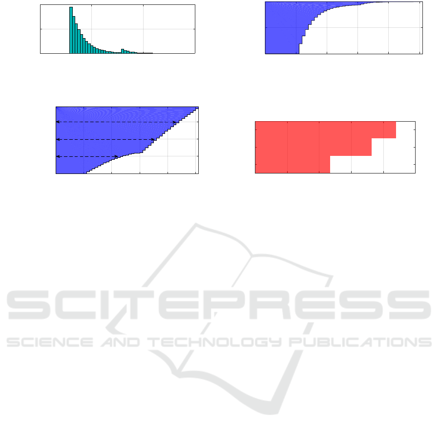
processing time t

0 20 40 60

Pr[T

= t]

0.1

0.2

(a) A discrete probability distribution over a set of

processing times.

processing time t

0 10 20 30 40 50

Pr[T

5 t]

0.5

(b) Corresponding cumulative distribution function.

processing time t

0 10 20 30 40 50

Pr[T

5 t]

0.9

0.99

0.999

(3)

(2)

(1)

processing time t

0 10 20 30 40 50

criticality level

(2)

(3)

(1)

(d) Resulting F-shaped task with X

= 3

Figure 2: Discretized cumulative distribution function forms an F-shaped task.

4 PROBLEM STATEMENT

We assume a set of non-preemptive F-shaped tasks

M C

= {T

,. .. , T

} to be processed on a single ma-

chine. We deﬁne an F-shaped task and its criticality

as follows:

Deﬁnition 1 (F-shape). The F-shape T

is a pair

) where X

∈ {1, . . ., L}, L ∈ N is the task crit-

icality and P

∈ N

, P

= (p

(1)

, p

(2)

,. .. , p

)

) is the

vector of processing times such that

(1)

< p

(2)

< . .. < p

)

The F-shape is an abstraction for non-preemptive

tasks with multiple different processing times. See

for example T

in Fig. 1. It is F-shaped task with crit-

icality X

= 3; therefore it has 3 different processing

times. Having a set I

M C

of F-shaped tasks, we deﬁne

the feasible schedule as follows:

Deﬁnition 2 (Feasible Schedule). By the schedule for

a set of F-shaped tasks I

M C

= {T

,. .. , T

} we re-

fer to an assignment (s

,. .. , s

) ∈ N

. We say that

schedule (s

,. .. , s

) for I

M C

is feasible if and only

if ∀i, j ∈ {1,. .. , n}, i 6= j :

+ p

(min{X

})

≤ s

) ∨ (s

+ p

(min{X

})

≤ s

Feasibility of a schedule with F-shaped tasks re-

quires that tasks do not overlap on any criticality level.

For example in Fig. 1, since T

follows after T

, it can-

not start earlier than s

+ p

(2)

, since min{X

} = 2

is the highest common criticality level of T

and T

We deal with the problem of ﬁnding a feasible

schedule for a set of F-shaped tasks with criticality

at most L such that the makespan (i.e. max s

+ p

)

is minimized. In the three-ﬁeld Graham-Blazewicz

notation it is denoted as 1|mc = L, mu|C

max

, where

mc = L stands for the mixed-criticality aspect of tasks

of maximal criticality L and mu stands for the match-

up. This problem is known to be N P -hard in the

strong sense even for mc = 2 (two criticality levels)

as shown by reduction from 3-Partition Problem in

(Hanzalek et al., 2016).

5 GENERAL PROPERTIES

Since the problem 1|mc = 2,mu|C

max

is strongly N P -

hard, it does not admit FPTAS unless P = N P . How-

ever, we show that the problem is polynomial-time

approximable within a constant multiplicative factor.

Proposition 1 (Approximability). For any given ﬁxed

L, the problem 1|mc = L,mu|C

max

is contained in

AP X complexity class.

Proof. Suppose the algorithm LCF (Least Criticality

First) that takes an input instance I

M C

and schedules

tasks in a non-decreasing sequence by their criticali-

ties without waiting. Then the makespan of resulting

schedule is

LCF(I

M C

) =

∑

i|X

(1)

∑

i|X

(2)

+ . . . +

∑

i|X

(L)

A sum of processing times on a given criticality level

over a set of tasks is a lower bound on the makespan.

ICORES 2017 - 6th International Conference on Operations Research and Enterprise Systems

164

Therefore we have

max{

∑

i|X

≥1

(1)

∑

i|X

≥2

(2)

,. .. ,

∑

i|X

≥L

(L)

} ≤

≤ OPT (I

M C

) ≤ LCF(I

M C

) ≤ L · OPT (I

M C

where OPT (I

M C

) denotes the optimal makespan of

M C

problem instance.

In fact, this result shows more than that there ex-

ists a polynomial-time algorithm producing schedules

with a constant bounded quality. For example, for

the problem with L = 2 criticality levels, actually any

left-shifted schedule will be at most twice as worse as

the optimal makespan since LCF actually produces

the worst ordering of tasks in terms of the makespan.

In the following sections, we present exact algo-

rithms for the problem with 2 and 3 criticality levels.

Due to the C

max

criterion, it can be shown that the

search for an optimal solution can be reduced to ﬁnd-

ing a permutation of tasks. Therefore, any optimal

schedule is given by a permutation of tasks π. Hence

we denote the makespan of the left-shifted schedule

of permutation π by C

max

(π). In Sec. 6 we give a

characterization of the set of optimal permutations for

problem 1|mc = 2, mu|C

max

and we introduce a MILP

model utilizing it. In Sec. 7, we introduce an opera-

tor acting on F-shapes, and we show how the optimal

solutions for problems with two and three criticality

levels are related.

6 TWO CRITICALITY LEVELS

We showed that optimal solutions to 1|mc =

L, mu|C

max

are given by a permutation π of tasks. For

the problem with two criticality levels, the optimal

permutations can be characterized more precisely. Let

us refer to tasks with criticality X

= 2 as HI-tasks

and tasks with criticality X

= 1 as LO-tasks. The

key structure of the optimal permutations are cover-

ing blocks:

Deﬁnition 3 (Covering Block). For any given fea-

sible schedule (s

,. .. , s

), a HI-task T

and a LO-

task T

we say that T

is covered by T

, denoted as

∈ cov(T

), if and only if s

+ p

(1)

≤ s

< s

+ p

(2)

The covering block B

is then the HI-task T

and the

set of all LO-tasks covered by T

See an example in Fig. 1. There T

is covering T

and T

. All these tasks form a covering block. Al-

though the deﬁnition of covering block given above

is meant for the problem with two criticality levels,

the notion of covering can be generalized for more

criticality levels. We assign a length to each covering

block. The length is given as the maximum between

the processing time p

(2)

of the HI-task T

and the sum

of processing times of tasks covered by T

plus the

processing time of T

at the ﬁrst level p

(1)

Proposition 2 (Covering Block Length). Given the

covering block B

, its length deﬁned as

max{p

(1)

∑

∈cov(T

)

(1)

, p

(2)

}

is invariant with respect to the ordering of LO-tasks

for which T

∈ cov(T

Clearly, the ordering of LO-tasks T

for which

∈ cov(T

) does not affect the block length since all

LO-tasks are running without waiting. Furthermore,

we say that task T

is fully covered by the block B

if B

= p

(2)

and T

∈ cov(T

). If exists a task cov-

ered by the block B

that is not fully covered, then

we say that B

is saturated. The makespan C

max

the schedule is given by a permutation of covering

blocks. However, actually any permutation of cover-

ing blocks contributes to the makespan by the same

amount; hence it is not subject to optimization.

Proposition 3 (Interchangebility). For every instance

of the problem 1|mc = 2, mu|C

max

there exists an opti-

mal solution that is given by an arbitrary permutation

of covering blocks.

A characterization of optimal solutions for 1|mc =

2,mu|C

max

directly follows from Proposition 2 and 3:

Corollary 1. The optimal solution for 1|mc =

2,mu|C

max

is given by an assignment of LO-tasks to

HI-tasks.

6.1 Covering MILP Model for

1|mc = 2, mu|C

max

The following MILP model relies on Corollary 1.

The model assigns LO-tasks to the HI-tasks in or-

der to form covering blocks such that the sum of their

lengths is the minimum. The decision variable x

i j

in-

dicates whether the LO-task T

is covered by the HI-

task T

; therefore if T

∈ cov(T

), then x

i j

= 1. The

makespan is then given by the sum of lengths of cov-

ering blocks and the sum of processing times of all

LO-tasks that are not covered.

min

∑

i|X

∑

j|X

(1)

(1 −

∑

i|X

i j

) (6.1)

s.t.

≥ p

(1)

∑

j|X

(1)

i j

∀i ∈ I

M C

(6.2)

≥ p

(2)

∀i ∈ I

M C

(6.3)

Exact Approach to the Scheduling of F-shaped Tasks with Two and Three Criticality Levels

165

∑

i|X

i j

≤ 1 ∀ j ∈ I

M C

(6.4)

where

∈ Z

∀i ∈ I

M C

i j

∈ {0, 1} ∀i ∈ I

M C

,∀ j ∈ I

M C

The main advantage of this model over the model

proposed by (Hanzalek et al., 2016) is that it has

much stronger linear relaxation. Further in Sec. 8 we

demonstrate its ability to solve an order of magnitude

larger instances.

7 THREE CRITICALITY LEVELS

Although two criticality levels are often sufﬁcient for

safety-critical application and this case is frequently

studied in the ﬁeld of mixed-critical systems (Burns

and Davis, 2013), sometimes the application natu-

rally contains three or more criticality levels. We cap-

ture the direct relation between problems with differ-

ent maximum criticality levels by introducing a trans-

formation given bellow. It is based on the obser-

vation that omitting some criticality levels provides

an instance of the problem with less criticality level

while maintaining a lower bound property. Further-

more, we introduce the Bottom-up algorithm that uses

this observation. The algorithm is used then together

with Covering MILP model for three criticality levels

(L = 3) shown in Sec. 7.2 to form an efﬁcient solution

method.

The transformation is deﬁned as h

restrictions:

Deﬁnition 4 (h

restrictions). Given the mixed-

criticality instance I

M C

and a positive integer h ∈ N,

let I

−

M C

and I

M C

be sets deﬁned as

−

M C

={(min{h,X

}, (p

(1)

,. .. , p

(min{h,X

})

)) |

∀i ∈ I

M C

}

M C

={(X

− h + 1, (p

(h)

,. .. , p

)

)) |

∀i ∈ I

M C

: X

≥ h}

We refer to I

−

M C

) as h

−

) restriction of the

instance I

M C

The h

−

restriction takes an F-shape and cuts off all

criticality levels above level h. Similarly, given the set

of F-shaped tasks, h

restriction drops all tasks with

criticality below h, and for the rest, it cuts off criti-

cality levels less than h. Restricting an I

M C

instance

yields to a mixed-criticality instance since omitting

some of the criticality levels for an F-shape gives us

an F-shape. The application of the restriction can be

viewed as a relaxation the problem.

Proposition 4 (Two Lower Bounds on the

Makespan). For the problem 1|mc = 3, mu|C

max

expressions lb

−

, lb

deﬁned as

= min

π∈Π(I

M C

)

max

(π)

are lower bounds on the makespan, where Π(I

M C

)

and Π(I

−

M C

) denote the set of all permutations of ele-

ments I

M C

, I

−

M C

respectively.

Proof. The lb

−

is a lower bound on the makespan of

1|mc = 3,mu|C

max

since it relaxes on the overlapping

condition at the third criticality level. Similarly, lb

a lower bound on the makespan since it relaxes on the

overlapping condition at the ﬁrst criticality level.

7.1 Bottom-up Algorithm

We introduce a heuristic algorithm for the problem

1|mc = 3, mu|C

max

. Let us refer to tasks with X

= 3

(i.e. criticality 3) as to GREAT-tasks. The Bottom-

up algorithm is based on the idea of constructing the

schedule in two stages. In the ﬁrst stage, the relaxed

problem is solved up to the optimality, which mini-

mizes a lower bound on the optimal makespan of the

original problem. The second stage takes the relaxed

solution and constructs a locally optimal solution for

the original problem.

The ﬁrst stage of the algorithm solves 2

−

restric-

tion of the given problem instance; hence it is an

instance of 1|mc = 2, mu|C

max

problem that can be

solved with the model described in Section 6. It as-

signs LO-tasks to HI-tasks and GREAT-tasks; there-

fore it forms covering blocks. In the second stage,

the algorithm deﬁnes a new problem instance I

M C

the problem 1|mc = 2, mu|C

max

. The instance is con-

structed as follows. It contains LO-tasks with process-

ing time equal to the length of covering blocks from

the stage one. LO-tasks that are not part of any cover-

ing block are assigned to an arbitrary covering block.

The assignment of LO-tasks to 2

−

restricted GREAT-

tasks from the ﬁrst stage deﬁnes HI-tasks in the new

instance I

M C

. Then, the I

M C

instance is solved once

again as an instance of 1|mc = 2, mu|C

max

problem.

See the complete description of the Bottom-up algo-

rithm in Alg. 1.

In general, the Bottom-up algorithm produces

suboptimal solutions even though they are provably

bounded by a factor of 3 from the optimal solution,

as stated by Proposition 1. However, there are cases

when we can verify if the produced schedule is opti-

mal. This is achieved by the concept of critical paths

that captures the cause of achieved makespan.

ICORES 2017 - 6th International Conference on Operations Research and Enterprise Systems

166

Algorithm 1: Bottom-up.

1: π ← solve I

−

M C

restriction by Covering MILP 6.1

2: I

M C

←

3: for each covering block B

in the left-shifted so-

lution π do

4: if X

= 2 in I

M C

then

5: P

← (B

)

6: I

M C

← I

M C

∪ {(1, P

)}

7: else if B

< p

(3)

then

8: P

← (B

, p

(3)

)

9: I

M C

← I

M C

∪ {(2, P

)}

10: else

11:  block B

is saturated, it contributes by a

constant term to the makespan of I

M C

12: end if

13: end for

14: π ← solve I

M C

by Covering MILP 6.1

Deﬁnition 5 (Critical Path). Given the left-shifted

schedule (s

,. .. , s

) of the permutation π, the critical

path is CP ⊆ {1,. .. , |

π|}×{1, . . ., L} for some

π ⊆ π

such that ∀(i, ) ∈ C P ,i < |

π| : s

π(i)

+ p

()

π(i)

= s

π(i+1)

where

∑

(i,)∈C P

()

π(i)

= C

max

(π) = C

max

(

π).

Essentially, for any given left-shifted schedule, the

critical path is a subset of tasks and their criticality

levels such that ∀(i, ) ∈ C P holds that if the process-

ing time p

()

π(i)

is increased by some ε > 0, then the

makespan of the same schedule is also increased by ε.

Proposition 5 (Sufﬁcient Optimality Conditions). If

one of following conditions holds, then the schedule

produced by the Bottom-up algorithm is optimal for

problem 1|mc = 3,mu|C

max

1. There exists a critical path going through the ﬁrst

and the second levels only.

2. Every LO-task is fully covered by the second crit-

icality level.

When none of the optimality conditions is satis-

ﬁed, e.g. a critical path is coming through every criti-

cality level, we get back to the MILP model 7.2 for the

problem 1|mc = 3, mu|C

max

in order to ﬁnd an optimal

solution or for the proof that the current solution is the

optimal one. The solver is supplied with the initial so-

lution and a lower bound obtained by the Bottom-up

algorithm. The computational time of Bottom-up al-

gorithm is dominated by lines 1 and 14. The total

computational times are reported in Tab. 2.

7.2 Covering MILP Model for

1|mc = 3, mu|C

max

The Covering MILP model for three criticality lev-

els uses a similar idea as the model for 1|mc =

2,mu|C

max

. It assigns LO-tasks to covering blocks

and covering blocks to the GREAT-tasks. The model

utilizes the idea that optimal solutions are made of

blocks (in this case formed by GREAT-tasks that cover

less critical tasks) whose order is interchangeable

within a solution. It assigns LO-tasks to the HI-tasks

and to 2

−

restriction of GREAT-tasks to form cover-

ing blocks. Blocks are assigned to the GREAT-tasks

in order to create a solution. The big M constant is

as large as the number of LO-tasks contained in the

problem instance.

min

∑

i|X

∑

j|X

∑

k|X

(1)

0,k

(7.1)

s.t.

≥ p

(3)

∀i ∈ I

M C

(7.2)

i, j

≥

∑

k|X

i, j,k

∀i ∈ I

M C

∪

0,∀ j ∈ I

M C

(7.3)

j,i

≥ p

(2)

i, j

∀i ∈ I

M C

∪

0,∀ j ∈ I

M C

(7.4)

j,i

≥ p

(1)

i, j

∑

k|X

(1)

i, j,k

∀i ∈ I

M C

∪

0,∀ j ∈ I

M C

(7.5)

≥ p

(2)

∑

j|X

j,i

∀i ∈ I

M C

(7.6)

≥ p

(1)

∑

j|X

j,i

∑

k|X

(1)

0,k

∀i ∈ I

M C

(7.7)

∑

i|X

=3∪

∑

j|X

=2∪

i, j,k

≥ 1

∀k ∈ I

M C

(7.8)

∑

i|X

=3∪

i, j

≥ 1 ∀ j ∈ I

M C

(7.9)

where

i, j

∈ {0, 1}∀i ∈ I

M C

∪

0,∀ j ∈ I

M C

i, j,k

∈ {0, 1}

∀i ∈ I

M C

∪

0,∀ j ∈ I

M C

∪

∀k ∈ I

M C

∪

0 : k 6=

0 ∨ (i =

0 ∧ j =

∈ Z

∀i ∈ I

M C

j,i

∈ Z

∀i ∈ I

M C

∪

0,∀ j ∈ I

M C

Exact Approach to the Scheduling of F-shaped Tasks with Two and Three Criticality Levels

167

When Bottom-up fails to prove optimality, it goes

back to this model while supplying the lb

−

lower

bound and the initial solution. The reason for exe-

cuting Bottom-up ahead solving MILP model 7.2 is

two-fold. First, we have observed the solver struggles

to prove optimality when the solution is clearly opti-

mal regarding the critical path. The other observation

is that if the problem instance contains the majority of

tasks with criticality one and two, then solving its 2

−

restriction frequently yields optimal solution since the

highest criticality levels are not likely to be utilized.

The same holds for the instances with a large number

of tasks with higher criticality. Furthermore, solving

restrictions of I

M C

is cheap compared to the solv-

ing the whole MILP model 7.2 as it can be seen in

Tab. 1.

8 COMPUTATIONAL

EXPERIMENTS

For the problem 1|mc = 2, mu|C

max

we have randomly

generated sets of 20 instances with n tasks for each

n ∈ {10, .. ., 200}. Criticalities of tasks were dis-

tributed uniformly. The processing time of a task

at level 1 is sampled from the uniform distribution

U(1,11). For tasks with the criticality of 2, the pro-

longation at level 2 is sampled from uniform distribu-

tion U(1,10).

For the problem 1|mc = 3, mu|C

max

we have ran-

domly generated sets of 20 instances with n tasks

for each n ∈ {10,. .. , 80}. For each n, the set con-

tains instances with different splits of tasks’ critical-

ities and different distributions for prolongation (e.g.

U(1,10) and U(1,7) for the second level, U(1, 10)

and U(1,14) for the third level, etc.) in order to gen-

erate instances of various properties. We have inves-

tigated the impact of different processing time dis-

tributions to the overall performance. We have ob-

served that the the proposed approach is not sensitive

to the choice of particular distributions, but rather to

the difference between combined processing times al-

located to each criticality level. Therefore, in our ex-

periments, we have used uniform distributions with

parameters that represent challenging instances.

The column avg t (max t) in Tab. 1 and 2 de-

notes the average (maximal) computational time for

instances that were solved within the time limit of

300 s. The column unsl contains the percentage of in-

stances that were not solved within the time limit and

avg gap denotes average optimality gap proven by the

solver for the unsolved instances. Results were ob-

tained with two Intel Xeon E5-2620 v2 @ 2.10 GHz

processors using Gurobi Optimizer 6.5 with the algo-

rithms implemented in Python 3.4.

In Tab. 1 it can be seen that our model is able to

solve about an order of the magnitude larger prob-

lem instances. The Relative Order model proposed

by (Hanzalek et al., 2016) consistently fails to narrow

optimality gap for instances with more than 40 tasks.

In Tab. 2 it is shown that the combination of Bottom-

up heuristic and MILP 7.2 is able to solve reliably in-

stances with 60 tasks up to the optimality and almost

all instances with 80 tasks. Moreover, the proven gap

is much smaller than for the Relative Order model;

therefore it shows that our model has stronger linear

relaxation.

To put our algorithms into the another test, we

tested them on data obtained from our automotive in-

dustrial partner. The data comes from a real-life au-

tomotive system consisting of a communication mes-

sages between 23 ECUs. From this instance, we con-

structed a probabilistic model that corresponds to the

given instance. We are interested in scheduling mes-

sages inside the basic period (10 ms); therefore those

are messages occurring in every communication cy-

cle. The aim is to minimize C

max

to maximize re-

maining space for other messages with larger periods.

The instance divides messages into three cate-

gories. The lowest critical are debug and develop-

ment messages which do not use any form of a check-

sum. More critical messages are secured by a par-

ity check. The most critical messages are secured

by CRC8 code. The message criticalities are dis-

tributed according Pr[X

= 1] = 0.48, Pr[X

= 2] =

0.48, Pr[X

= 3] = 0.04. The length of each mes-

sage is drawn from distribution U(8,12). The pro-

longation on the second and the third criticality level

is sampled from U(8, 16) to model the message re-

transmission and an extra overhead.

The real-life industrial dataset was created by gen-

erating 20 instances of the problem 1|mc = 3,mu|C

max

according to distributions mentioned above for each

of n ∈ {50, 100, 150, 200}, where n is the number of

messages. The results are reported in Tab. 3. The

computational times were obtained under the same

circumstances as described above.

The results for real-life industrial data are quanti-

tatively better compared to those obtained in Tab. 2.

The reason is likely that the data contain relatively

a few GREAT-tasks and the range of lengths of LO-

tasks is relatively narrow. Therefore, many of them

are identical, and the solver might be able to exploit

this symmetry even though it was not supplied to it.

With the Covering MILP model, the solver scales well

even for larger instances.

ICORES 2017 - 6th International Conference on Operations Research and Enterprise Systems

168

Table 1: Computational results for the problem 1|mc = 2, mu|C

max

Covering MILP 6.1 Relative Order MILP (Hanzalek et al., 2016)

n tasks avg t [s] max t [s] unsl [%] avg gap [%] avg t [s] max t [s] unsl [%] avg gap [%]

10 > 0.01 0.03 0 — 13.07 (±44.93) 200.22 0 —

15 > 0.01 0.03 0 — 49.67 (±49.38) 127.09 60 27.32 (±12.54)

20 0.01(±0.01) 0.03 0 — — — 100 40.09 (±15.27)

40 0.09(±0.17) 0.81 0 — — — 100 77.66(±6.23)

60 1.37(±4.33) 19.71 0 — — — 100 84.23(±2.90)

80 0.38(±0.45) 1.94 0 — — — 100 90.72(±1.77)

100 1.28(±1.38) 5.05 0 — — — 100 93.38(±0.76)

150 11.77 (±24.29) 93.01 0 — — — 100 96.02(±0.24)

200 22.69 (±61.24) 281.04 0 — — — 100 97.33 (±0.13)

Table 2: Computational results for the problem 1|mc = 3, mu|C

max

Bottom-up w/ Covering MILP 7.2 Relative Order MILP (Hanzalek et al., 2016)

n tasks avg t [s] max t [s] unsl [%] avg gap [%] avg t [s] max t [s] unsl [%] avg gap [%]

10 0.02 (±0.01) 0.04 0 — 0.09 (±0.07) 0.28 0 —

20 0.16 (±0.36) 1.66 0 — — — 100 28.71 (±16.62)

30 0.17 (±0.17) 0.66 0 — — — 100 63.28 (±7.35)

40 0.69 (±1.02) 3.61 0 — — — 100 72.85 (±6.14)

50 2.40 (±7.42) 33.56 0 — — — 100 80.61(±2.96)

60 6.71(±11.97) 44.67 0 — — — 100 84.30 (±2.70)

70 11.30(±22.31) 79.38 10 0.38 (±0.19) — — 100 89.34(±1.43)

80 37.92(±68.82) 224.86 20 0.34 (±0.13) — — 100 91.09(±1.40)

Table 3: Computational results for the real-life instances.

Bottom-up w/ Covering MILP 7.2

n tasks avg t [s] avg gap [%]

50 0.08(±0.14) —

100 1.17(±3.33) —

150 3.67(±7.23) 0.26 (±0.00)

200 5.34(±15.51) —

9 CONCLUSION

In this paper, we have proposed two exact approaches

for the problem of non-preemptive mixed-criticality

match-up scheduling for solving the problem of mes-

sage retransmission in time-triggered communication

protocols. We investigated the fundamental proper-

ties of F-shapes to obtain efﬁcient models of the prob-

lem. Our algorithms outperform recently proposed

approach by a large margin. Furthermore, we showed

the membership of 1|mc = L, mu|C

max

problem in

AP X complexity class for an arbitrary ﬁxed L.

ACKNOWLEDGEMENT

This work was supported by the Grant Agency of

the Czech Republic under the Project GACR P103-

16-23509S. Furthermore, this work was supported

by the US Department of the Navy Grant N62909-

15-1-N094 SALTT issued by Ofﬁce Naval Research

Global. The United States Government has a royalty-

free license throughout the world in all copyrightable

material contained herein.

REFERENCES

Baruah, S. and Fohler, G. (2011). Certiﬁcation-cognizant

time-triggered scheduling of mixed-criticality sys-

tems. In Real-Time Systems Symposium (RTSS), 2011

IEEE 32nd, pages 3–12. IEEE.

Baruah, S., Li, H., and Stougie, L. (2010). Towards the

design of certiﬁable mixed-criticality systems. In

Real-Time and Embedded Technology and Applica-

tions Symposium (RTAS), 2010 16th IEEE, pages 13–

22. IEEE.

Bean, J. C., Birge, J. R., Mittenthal, J., and Noon, C. E.

(1991). Matchup scheduling with multiple resources,

release dates and disruptions. Operations Research,

39(3):470–483.

Bell, R. (2006). Introduction to iec 61508. In Proceedings

of the 10th Australian workshop on Safety critical sys-

tems and software-Volume 55, pages 3–12. Australian

Computer Society, Inc.

Bertsimas, D., Brown, D. B., and Caramanis, C. (2011).

Theory and applications of robust optimization. SIAM

review, 53(3):464–501.

Burns, A. and Davis, R. (2013). Mixed criticality systems-a

review. Department of Computer Science, University

of York, Tech. Rep.

Dvorak, J. and Hanzalek, Z. (2016). Using two indepen-

dent channels with gateway for FlexRay static seg-

Exact Approach to the Scheduling of F-shaped Tasks with Two and Three Criticality Levels

169

ment scheduling. IEEE Transactions on Industrial In-

formatics, article in press.

Hanzalek, Z., Tunys, T., and Sucha, P. (2016). Non-

preemptive mixed-criticality match-up schedul-

ing problem. Journal of Scheduling, doi:

10.1007/s10951-016-0468-y.

Kopetz, H., Ademaj, A., Grillinger, P., and Steinhammer,

K. (2005). The time-triggered ethernet (TTE) design.

In Object-Oriented Real-Time Distributed Computing,

2005. ISORC 2005. Eighth IEEE International Sym-

posium on, pages 22–33. IEEE.

Qi, X., Bard, J. F., and Yu, G. (2006). Disruption manage-

ment for machine scheduling: the case of spt sched-

ules. International Journal of Production Economics,

103(1):166–184.

Sahinidis, N. V. (2004). Optimization under uncertainty:

state-of-the-art and opportunities. Computers &

Chemical Engineering, 28(6):971–983.

Shabtay, D., Gaspar, N., and Kaspi, M. (2013). A survey on

ofﬂine scheduling with rejection. Journal of schedul-

ing, 16(1):3–28.

Theis, J., Fohler, G., and Baruah, S. (2013). Schedule ta-

ble generation for time-triggered mixed criticality sys-

tems. Proc. WMC, RTSS, pages 79–84.

Vestal, S. (2007). Preemptive scheduling of multi-criticality

systems with varying degrees of execution time assur-

ance. In Real-Time Systems Symposium, 2007. RTSS

2007. 28th IEEE International, pages 239–243. IEEE.

ICORES 2017 - 6th International Conference on Operations Research and Enterprise Systems

170

REFERENCES

Baruah, S. and Fohler, G. (2011). Certification-cognizant