
Acoustic Detection of Violence in Real and Fictional Environments
Marta Bautista-Dur
´
an, Joaqu
´
ın Garc
´
ıa-G
´
omez, Roberto Gil-Pita, H
´
ector S
´
anchez-Hevia,
Inma Mohino-Herranz and Manuel Rosa-Zurera
Signal Theory and Communications Department, University of Alcal
´
a, 28805 Alcal
´
a de Henares, Madrid, Spain
{marta.bautista, joaquin.garciagomez}@edu.uah.es
Keywords:
Violence Detection, Audio Processing, Feature Selection, Real Environment, Fictional Environment.
Abstract:
Detecting violence is an important task due to the amount of people who suffer its effects daily. There is a
tendency to focus the problem either in real situations or in non real ones, but both of them are useful on
its own right. Until this day there has not been clear effort to try to relate both environments. In this work
we try to detect violent situations on two different acoustic databases through the use of crossed information
from one of them into the other. The system has been divided into three stages: feature extraction, feature
selection based on genetic algorithms and classification to take a binary decision. Results focus on comparing
performance loss when a database is evaluated with features selected on itself, or selection based in the other
database. In general, complex classifiers tend to suffer higher losses, whereas simple classifiers, such as linear
and quadratic detectors, offers less than a 10% loss in most situations.
1 INTRODUCTION
The term of violence has a subjective connotation, but
one definition extracted from The World Health Or-
ganization defined violence as “the intentional use of
physical force or power, threatened or actual, against
oneself, another person, or against a group or commu-
nity, which either results in or has a high likelihood of
resulting in injury, death, psychological harm, malde-
velopment, or deprivation” (Krug et al., 2002). There
are many more valid definitions, such as “physical vi-
olence or accident resulting in human injury or pain”
(Demarty et al., 2012), “a series of human actions
accompanying with bleeding” (Chen et al., 2011) or
“any situation or action that may cause physical or
mental harm to one or more persons” (Giannakopou-
los et al., 2006). In the context of this work the kind of
actions that will be consider as violence are shouting
and hits.
Violence can take place in multiple environments
and in multiple ways. It is important to obtain a
method capable of detecting violent situations on their
early stages with the aim of stopping them or prevent-
ing them from escalating.
Some related work on the literature is based on
multimedia contest, such as (Demarty et al., 2012),
(Xu et al., 2005), or (Nam et al., 1998), where the
database is composed by audio and video signals ex-
tracted from movies. With a mixed setup it is possi-
ble to detect violent content from ‘bloody’ scenes, or
simply from the behavior of people extracted from the
video. If the task is to detect violence in real environ-
ments, using cameras entails a privacy intrusion that
can be avoided using audio alone. That is why our
purpose is evaluating only the audio.
These studies have been done using pretended vi-
olence from films, although can distort the general-
ization of the results when presented with actual vio-
lence. Violence detection is an emerging field related
with smart cities. For that reason the objective in this
work is to evaluate the results when data from both
real and pretended scenarios is combined.
In this paper two different kinds of violence have
been considered. On the one hand, actual violent sit-
uations where the audio has been taken from records
directly from real recordings. On the other hand, fic-
tional situations, where the data is composed of vari-
ous audio clips extracted from film scenes. The possi-
ble applications of violence detection in real scenarios
have been explained in detail in (Garc
´
ıa-G
´
omez et al.,
2016). Fictional violence detection can be a useful
tool for content tagging on videogames or movies, in
order to secure child protection.
There are some reasons why we have distin-
guished between these two situations. One of them is
that in real scenarios the signals are not preprocessed,
unlike fictional scenarios where the signals are heav-
ily modified by different factors. This preprocessing
456
Bautista-Durán, M., García-Gómez, J., Gil-Pita, R., Sánchez-Hevia, H., Mohino-Herranz, I. and Rosa-Zurera, M.
Acoustic Detection of Violence in Real and Fictional Environments.
DOI: 10.5220/0006195004560462
In Proceedings of the 6th International Conference on Pattern Recognition Applications and Methods (ICPRAM 2017), pages 456-462
ISBN: 978-989-758-222-6
Copyright
c
2017 by SCITEPRESS – Science and Technology Publications, Lda. All rights reserved
FEATURE
EXTRACTION
VIOLENCE
DETECTION
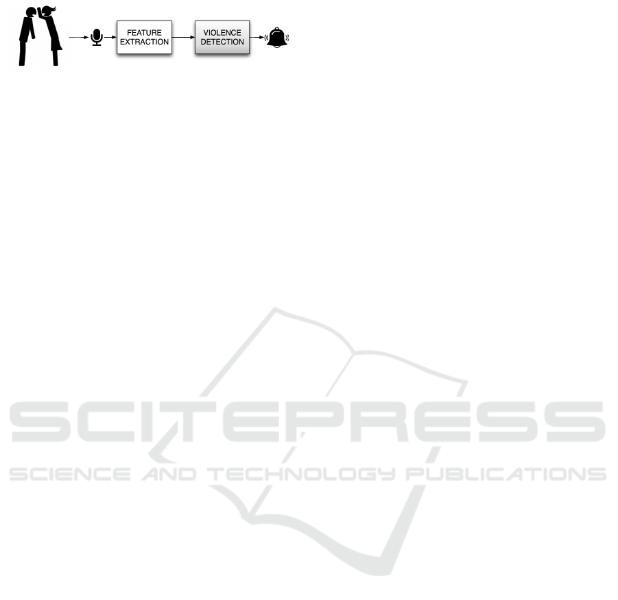
Figure 1: Proposed system.
modifies the properties of the audio signal. Another
reason is the different situation in where they take
place. In real environments the sound is very different
to than on fictional ones, hits or speech in real envi-
ronments may have background noise and the speech
loudness varies over time. Movies recreate sound as
much as the actions taking place on screen. Audio
tracks are commonly composed of a series of care-
fully chosen sounds with the main objective of being
pleasing to the ear. The objective of this paper is to
evaluate the performance of a single violence detec-
tion system when exposed to sounds coming from two
sources. This will be explained in detail below.
This paper is structured as follows. First, Sec-
tion 2 introduces the implemented detector system,
the feature extraction (Subsection 2.1) and the feature
selection (Subsection 2.2). Then, Section 3 describes
the experiments and results, including the description
of the database (Subsection 3.1), the description of
the experiments (Subsection 3.2) and the discussion
of the results (Subsection 3.3). Finally, Section 4
presents the conclusions.
2 PROPOSED SYSTEM
The proposed system has the aim of resolving the vi-
olence detection problem in both real and fictional
environments on its own, as well as comparing the
performance when they are combined. As we previ-
ously stated, the system will be only based on audio,
which will be processed to extract useful information
and then the data will be classified to make a deci-
sion every T seconds. In Figure 1 the scheme of the
system is proposed.
In this study three different classifiers will be
tested: a Least Squares Linear Detector (LSLD), a
simplified version of Least Squares Quadratic Detec-
tor (LSQD) and a Neural Network based Detector
with 5 hidden neurons. All of them are explained in
detail in (Garc
´
ıa-G
´
omez et al., 2016).
2.1 Feature Extraction
The objective of the feature extraction is to process
the input audio signal in order to obtain useful infor-
mation that helps the classifying algorithm to properly
detect violent situations. Features have been evalu-
ated in frequency or time domain. In order to evalu-
ate these features, the audio segments have been di-
vided into S frames of 400 ms length with an overlap
of 95%. The evaluated features are:
• Mel-Frecuency Cepstral Coefficients (MFCCs)
Mel-Frecuency Cepstral Coefficients have been
computed from the Short Time Fourier Transform
(STFT). MFCCs is commonly used in speech
recognition due to the fact that Mel scale divides
the frequency bands in a similar way to the human
ear. The information provided by this feature is a
compact representation of the spectral envelope,
so most of the signal energy is located in the first
coefficients. We are using 25 coefficients. The
statistics applied to this feature are: mean, stan-
dard deviation (std), maximum (max) and median
(these two last only in some MFCCs).
• Delta Mel-Frequency Cepstral Coefficients
(∆MFCCs)
This feature is extracted from the previous one,
and represent the difference between two MFCCs.
The implementation details are presented in (Mo-
hino et al., 2013). The statistics applied to this
feature are: mean and standard deviation.
• Pitch
Also named fundamental frequency, this feature
determines the tone of the speech and can be used
to distinguish between persons (Gil-Pita et al.,
2015). In order to get this measure, the prediction
error is obtained by filtering the audio frames with
the linear prediction coefficients and then the au-
tocorrelation of the error is evaluated. If the value
of peaks in the autocorrelation is 20% higher than
the maximum of the autocorrelation, the frame
will be considered as voiced, otherwise unvoiced
(Mohino et al., 2013) The statistics applied to this
measure are: mean and standard deviation.
• Harmonic Noise Rate (HNR)
Harmonic Noise Rate measures the relationship
between the harmonic energy produced by the vo-
cal cords versus non-harmonic energy present in
the signal (Mohino et al., 2011). The statistics
applied to this measure are: mean and standard
deviation.
• Short Time Energy (STE)
Short Time Energy is the energy of a short speech
segment. This parameter is considered a good fea-
ture to differentiate between voiced and unvoiced
frames (Jalil et al., 2013). The statistics applied to
this measure are: mean and standard deviation.
Acoustic Detection of Violence in Real and Fictional Environments
457

• Energy Entropy (EE)
The Energy Entropy expresses abrupt changes in
the energy level of the audio signal. This is useful
for detecting violence due to rapid changes occur-
ring in the tone of voice. To obtain this parameter
the frames are subdivided into small subframes.
The statistics applied to this measure are: mean,
standard deviation, maximum, ratios of maximum
to mean and maximum to median value.
• Zero Crossing Rate (ZCR)
Zero Crossing Rate shows how quickly the power
spectrum of a signal fram is changing in relation
to the previous one (Giannakopoulos et al., 2006).
The statistics applied to this measure are: mean
and standard deviation.
• Spectral Flux (SF)
This feature is evaluated in the frequency domain.
It represents the squared difference between the
normalized magnitudes of successive spectral dis-
tributions (Tzanetakis and Cook, 2002). The
statistics applied to this measure are: mean and
standard deviation.
• Spectral Rolloff (SR)
This measure represent the skewness of the spec-
tral shape (Giannakopoulos et al., 2006). It is
defined as the frequency below which a percent-
age of the magnitude distribution of the Discrete
Fourier Transform (DFT) coefficients are con-
centrated for frame. Different information can
be extracted from music, speech or gunshots,
so it might be interesting for violence detection
(Garc
´
ıa-G
´
omez et al., 2016). The statistics ap-
plied to this measure are: mean and standard de-
viation.
• Spectral Centroid (SC)
Spectral Centroid studied in the frequency domain
is defined as the center of gravity of the magni-
tude spectrum of the STFT (Tzanetakis and Cook,
2002). The statistics applied to this measure are:
mean and standard deviation.
• Ratio of Unvoiced Time Frames (RUF)
This value is associated to the presence or ab-
sence of strong speech in the analyzed audio. For
that, the amount of unvoiced frames is evaluated
(Garc
´
ıa-G
´
omez et al., 2016).
• Spectrum (SP)
This measure corresponds to the DFT of the signal
(Doukas and Maglogiannis, 2011). The statistics
applied to this measure are: maximum and stan-
dard deviation.
2.2 Selecting Features
In order to select the best features, we have resorted
to a Genetic Algorithm (GA), which is based on the
random exchange of features between the individuals
of a population. This population represents the pos-
sible set of solutions for the problem. GA involves
four steps: creation of the population, individual se-
lection, crossover and mutation. After the first itera-
tion, the algorithm goes back to the selection step and
repeats cyclically. The parameter to be optimized is
the probability of detection for a given probability of
false alarm. In order to maximize this value, features
are ranked according to their performance. By using
only the best features the performance will increase
and the computational cost of the implementation will
decrease. The classifiers used in the optimization
process were LSLD and LSQD as in (Garc
´
ıa-G
´
omez
et al., 2016), to soften the computational cost, which
is far less than employing neural networks.
The parameters used are the same than in (Garc
´
ıa-
G
´
omez et al., 2016): 51 total features, 20 selected fea-
tures, 100 individuals, 10 parents, 90 generated sons,
a probability of mutation of 4%, 30 iterations and 10
repetitions of the GA.
3 EXPERIMENTS AND RESULTS
The main objective of the paper is to study the rela-
tion between actual violence and violence recreations
from movies. Because of that, a set of experiments
has been carried out using two different databases,
both sampled to a frequency of 22,050 Hz and com-
posed of audio segments of 5 seconds length. Frame
length was selected due to its performance when com-
pared to other values.
3.1 Database Description
In order to carry out the experiments of this paper, we
need two different databases: one composed of real
world audio and another from films. The first one was
developed in (Garc
´
ıa-G
´
omez et al., 2016), so we will
use the same to ease a comparison. The details of this
database are summarized in Table 1.
The new database shares the most its important
properties with the old one, such as the amount of per-
centage of violence (around 10%) and the sampling
frequency (22,050 Hz). The film database is com-
posed of small extracts from films (between tenths of
seconds and a few minutes), labeled according to the
kind of content in as to indicate when a violent situ-
ation is taking place. The summarized properties are
ICPRAM 2017 - 6th International Conference on Pattern Recognition Applications and Methods
458

Table 1: Summary of the real world database.
Parameters Value
Total duration 27,802 s
Violence duration 3,051 s
Percentage of violence 10.97%
Number of fragments 109
Minimum audio length 1.51 s
Maximum audio length 4,966 s
Table 2: Summary of the movie database.
Parameters Value
Total duration 15,701 s
Violence duration 1,466 s
Percentage of violence 9.34%
Number of fragments 902
Number of films 119
Minimum audio length 15 s
Maximum audio length 126.30 s
detailed in Table 2. In order to get a database suitable
for a general study, many film genres have been in-
cluded in the database, such as: action (Aliens, The
Avengers, The Dark Knight), comedy (Anchorman,
Balls of Fury, You, me and Dupree), fantasy (Avatar,
The Chronicles of Narnia, Harry Potter and the Half-
Blood Prince), drama (Braveheart, Cast Away, Get-
tysburg), horror (I know what you did last summer,
The Ring, Red Dawn) and others.
3.2 Description of the Experiments
In this study two different kinds of experiments are
considered. First the system is trained and tested with
one of the databases, then the databased are crossed.
That is to say, the training step is performed with the
real database and the test step with the fictional one,
or vice versa. The procedure when only one database
is used is explained in detail in (Garc
´
ıa-G
´
omez et al.,
2016), Section 3. For this study, the same process has
been done over the film database.
Figure 2 shows a block diagram which describes
the process carried out in the experiment using both
databases.
In case both databases are used for the experiment,
the process differs beyond the feature extraction pro-
cess. The training set is composed by one database
and the test set by the other one, so the classification
process is completely different.
In this case, feature selection has been done with
the whole database, while in the previous case we ap-
plied k − f old cross-validation, so all but of the sub-
sets were used (Garc
´
ıa-G
´
omez et al., 2016).
The way to extract the best features is the same
in the two experiments: the k − f old cross-validation
process is done in both cases to avoid generalization
EXTRACTING
THE AUDIO
FRAMES
FEATURE
EXTRACTION
TRAINING
SET
TEST SET
SELECTING
BEST
FEATURES
CLASSIFYING
FINAL
DECISION
DATABASE 1 DATABASE 2
DATABASE 1
Figure 2: Block diagram of the experiments.
loss and the classification methods used are the same,
LSLD and LSQD. The division of the film database
has been done in K subsets. The set of signals of each
film corresponds to 1 subset.
The selected features are then applied to the train-
ing set (composed by the same database), and the test
step is done over the other database. This classifi-
cation process differs from the previous one because
there is not k − f old cross-validation process due to
the use of two databases. In the previous experiment
only one database was available and this step was use-
ful to mantain generalization.
3.3 Results Discussion
This section will show the results obtained from the
experiments explained in previous sections. We will
mainly focus in two parameters: the probability of de-
tection as a function of the probability of false alarm
and the selected features for both databases.
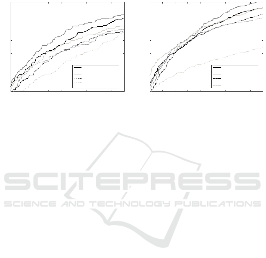
Figure 3 shows the Probability of Detection versus
the probability of False Alarm obtained for different
classifiers with the films database. The solid line cor-
responds to the movie-based training while the dashed
line represents the training with real signals.
Acoustic Detection of Violence in Real and Fictional Environments
459
1 2 3 4 5 6 7 8 9 10
Probability of False Alarm (%)
10
20
30
40
50
60
70
80
Probability of Detection (%)
Linear FS and LSLD
Quadratic FS and LSQD
Linear FS and MLP
Linear FS and LSLD
Quadratic FS and LSQD
Linear FS and MLP
Figure 3: Probability of Detection versus Probability of
False Alarm obtained for the film database.
As it might be expected, the best results are ob-
tained when the same database is used both in train-
ing and test (solid line). The best performance cor-
responds to the Quadratic Feature Selection (FS) and
LSQD, followed by the Linear FS and LSLD. When
the real world database is used to train, the relative
performance of the detectors is similar.
Nevertheless, the most important aspect is to com-
pare the performance when using a single database or
when crossing them. This is shown on Table 3, where
the probability of detection in function of some low
significant probabilities of false alarm (2%, 5% and
10%) is displayed. We distinguish between training
and testing with the same database or crossing them.
The loss parameter represents how the performance
decreases when using different databases and the av-
erage loss parameter is used to compare the different
classifiers applied to the set of probabilities of false
alarm.
In view of the results obtained here, the linear de-
tector is more resistant to database changes, since the
average loss in the set probabilities of false alarm is
approximately 7%. The quadratic detector and the
one based in Neural Networks have a similar behav-
ior, with losses higher tan 10%. If we focus in low
probabilities of false alarm (2% and 5%), the linear
detector works better than the others, with a loss of
5.70% and 5.26%. Interestingly, Neural Networks are
the best option for higher probabilities of false alarm
(10%), with a loss of only 4.82%.
Now we will focus in the other crossover be-
tween databases. Figure 4 shows the Probability of
Detection versus the Probability of False Alarm ob-
tained for the different classifiers with the real world
database. The solid line corresponds to real world
database based training while the dashed line repre-
1 2 3 4 5 6 7 8 9 10
Probability of False Alarm (%)
10
20
30
40
50
60
70
80
Probability of Detection (%)
Linear FS and LSLD
Quadratic FS and LSQD
Linear FS and MLP
Linear FS and LSLD
Quadratic FS and LSQD
Linear FS and MLP
Figure 4: Probability of Detection versus Probability of
False Alarm obtained for real world database.
sents films database based training. The latter can be
very interesting for the situations where we do not
have access to violent data in the real world and we
have to design the algorithm using films, video-games
or other substitutes.
As in movie-based violence, the best results are
obtained when the same database is used for the train-
ing and test steps (solid line). The best option is the
Quadratic FS and LSQD, followed by the Linear FS
and LSLD, and the same happens when training with
the other database. In this way, the results are essen-
tially the same in both cases.
Table 4 represents the performance loss of the real
world database results when using different databases
for training and test, in the same way as it was done
for the films database.
It is possible to see that LSLD is the best de-
tector again, with a loss of only 4.46% in average.
LSQD works great too, especially for low probabili-
ties (1.29% loss for 2% false alarm and 3.87% loss for
5% false alarm). Regarding the neural network based
detector, overfitting makes the average loss higher
than 26%.
If we compare the previous figures and tables, it
can be deduced that Neural Networks are not recom-
mended when databases are crossed during training
and test steps because the results have a poor perfor-
mance. It is more reliable to use linear or quadratic
detectors, depending on the probability of false alarm
we are interested in and the database used for training.
In order to compare the feature selection with both
databases, Tables 5 and 6 show the most selected fea-
tures in the films database for the linear FS process
and the quadratic FS process, ranked by the occur-
rence percentage (Occ. %). Shaded rows indicate the
repeated features in both real and films database.
ICPRAM 2017 - 6th International Conference on Pattern Recognition Applications and Methods
460

Table 3: Comparative results for different database usage during training.
Classifier Linear Quadratic MLP
Pfa (%) 2 5 10 2 5 10 2 5 10
Pd (%) - Films Training, Films Test 24.12 46.49 67.54 28.95 53.95 70.18 23.68 46.05 61.40
Pd (%) - Real Training, Films Test 18.42 41.23 57.46 22.37 41.23 58.77 10.96 30.70 56.58
Loss (%) 5.70 5.26 10.08 6.58 12.72 11.41 12.72 15.35 4.82
Average loss (%) 7.01 10.24 10.96
Table 4: Comparative results for different database usage during training.
Classifier Linear Quadratic MLP
Pfa (%) 2 5 10 2 5 10 2 5 10
Pd (%) - Real Training, Real Test 32.42 55.97 75.48 31.61 59.68 81.45 37.58 59.52 76.13
Pd (%) - Films Training, Real Test 25.48 54.35 70.65 30.32 55.81 67.74 17.74 31.29 44.52
Loss (%) 6.94 1.62 4.83 1.29 3.87 13.71 19.84 28.23 31.61
Average loss (%) 4.46 6.29 26.56
Considering this information we can appreciate
that the most useful features are quite different for
both databases. This is especially remarkable with the
linear FS, where only 6 of 20 features match, while
in the quadratic FS this number is increased to 12.
From this data it can be inferred that the linear FS is
more dependent on the used database with regard to
feature selection process than the quadratic FS, which
can successfully use 12 features for the two databases.
Focusing on common features, the robustness of
some of the features can be appreciated, such as
MFCCs and ∆MFCCs, pitch, short time energy or en-
ergy entropy. Concerning MFCCs and ∆MFCCs, 3
features match in the databases for the LSLD and 4
for the LSQD, representing a large amount of the total
features. It is noted that most of these are calculated
as standard deviation statistics. Pitch features are very
important because in the two detectors mean and/or
standard deviation appear with a 100% percentage of
occurrence. In respect of energy features, short time
energy is relevant for the two detectors, while energy
entropy ranks highly (7th and 8th) only in the LSQD.
It is also of interest to point out that the proposed
feature in (Garc
´
ıa-G
´
omez et al., 2016) ranks at the
top of the LQSD list and 10th in the LSLD list. Fur-
thermore, the appearance of features related to Har-
monic Noise Rate and Spectrum in the films database
is remarkable, which were not selected with the real
one. In addition, results show that features like spec-
tral centroid, spectral rolloff or spectral flux are not
useful in films, in contrast to the real world situations.
If we compare Tables 5 and 6, we can appreci-
ate that 14 of the total features are the same in both
tables, exactly the same number that it was obtained
in (Garc
´
ıa-G
´
omez et al., 2016) for real database. It
demonstrates once again that many of the statistics
can be applied in both quadratic and linear detectors.
Table 5: Summary of the selected features for the LSLD.
No. Measure Statistic Occ. (%)
1 MFCC 4 Mean 100.00
2 Pitch Mean 100.00
3 ∆MFCC 3 Std 98.20
4 ZCR Std 95.50
5 MFCC 1 Std 93.69
6 Pitch Std 93.69
7 MFFC 2 Mean 90.09
8 ∆MFCC 2 Std 90.09
9 MFCC 5 Std 88.29
10 RUF - 86.49
11 SP Mean 84.68
12 MFCC 3 Mean 75.68
13 STE Mean 62.16
14 HNR Mean 61.26
15 ∆MFCC 4 Std 60.36
16 EE Maximum 57.66
17 STE Std 38.74
18 MFCC 5 Mean 37.84
19 MFCC 3 Median 36.94
20 EE Max/Median 32.43
4 CONCLUSION
The purpose of this paper is to examine the viabil-
ity of violence detection on real audio recording with
a system trained using fictional data, and vice versa.
This differentiation is made because recording con-
ditions and audio preprocessing is different from one
environment to the other. This approach could be in-
teresting in case there is not enough available data for
a given scenario. Another possible application could
be to transfer the research efforts validated in one en-
vironment to another one.
The results with database crossover bring us a
similar conclusion: an increase of classifier complex-
ity implies a higher performance loss. Specifically,
linear detectors works better than quadratic detectors,
Acoustic Detection of Violence in Real and Fictional Environments
461

Table 6: Summary of the selected features for the LSQD.
No. Measure Statistic Occ. (%)
1 Pitch Mean 100.00
2 Pitch Std 100.00
3 RUF - 100.00
4 MFFC 4 Mean 99.10
5 MFCC 5 Std 97.30
6 HNR Mean 84.68
7 EE Std 84.68
8 EE Max/Median 83.78
9 SP Mean 83.78
10 MFCC 3 Mean 82.88
11 MFCC 1 Std 78.38
12 ZCR Max/Mean 78.38
13 STE Std 66.67
14 ∆MFCC 5 Std 55.86
15 EE Mean 52.25
16 ∆MFCC 1 Std 51.35
17 STE Mean 48.65
18 ∆MFCC 3 Std 46.85
19 MFCC 1 Mean 43.24
20 MFCC 5 Mean 37.84
and quadratic detectors better than those based on
neural networks. This can be explained by the fact
that the loss of generalization is directly related to
overfitting tendencies. In that way, neural networks
can work better for a specific environment (real or fic-
tional), or when a single database is used for training
and test. However, they are not able to get good re-
sults when the databases are crossed.
Future work will focus on using other types
of classifiers and testing the system with different
databases (e.g. videogames). The use of additional
features and statistics will also be explored.
ACKNOWLEDGEMENTS
This work has been funded by the Spanish Ministry
of Economy and Competitiveness (under project
TEC2015-67387-C4-4-R, funds Spain/FEDER)
and by the University of Alcal
´
a (under project
CCG2015/EXP-056).
REFERENCES
Chen, L.-H., Hsu, H.-W., Wang, L.-Y., and Su, C.-W.
(2011). Violence detection in movies. In Computer
Graphics, Imaging and Visualization (CGIV), 2011
Eighth International Conference on, pages 119–124.
IEEE.
Demarty, C.-H., Penet, C., Gravier, G., and Soleymani,
M. (2012). The mediaeval 2012 affect task: violent
scenes detection. In Working Notes Proceedings of
the MediaEval 2012 Workshop.
Doukas, C. N. and Maglogiannis, I. (2011). Emergency
fall incidents detection in assisted living environments
utilizing motion, sound, and visual perceptual compo-
nents. IEEE Transactions on Information Technology
in Biomedicine, 15(2):277–289.
Garc
´
ıa-G
´
omez, J., Bautista-Dur
´
an, M., Gil-Pita, R.,
Mohino-Herranz, I., and Rosa-Zurera, M. (2016). Vi-
olence detection in real environments for smart cities.
In Ubiquitous Computing and Ambient Intelligence:
10th International Conference, UCAmI 2016, San
Bartolom
´
e de Tirajana, Gran Canaria, Spain, Novem-
ber 29–December 2, 2016, Part II, pages 482–494.
Springer.
Giannakopoulos, T., Kosmopoulos, D., Aristidou, A., and
Theodoridis, S. (2006). Violence content classifica-
tion using audio features. In Hellenic Conference on
Artificial Intelligence, pages 502–507. Springer.
Gil-Pita, R., L
´
opez-Garrido, B., and Rosa-Zurera, M.
(2015). Tailored mfccs for sound environment clas-
sification in hearing aids. In Advanced Computer
and Communication Engineering Technology, pages
1037–1048. Springer.
Jalil, M., Butt, F. A., and Malik, A. (2013). Short-time en-
ergy, magnitude, zero crossing rate and autocorrela-
tion measurement for discriminating voiced and un-
voiced segments of speech signals. In Technological
Advances in Electrical, Electronics and Computer En-
gineering (TAEECE), 2013 International Conference
on, pages 208–212. IEEE.
Krug, E. G., Mercy, J. A., Dahlberg, L. L., and Zwi, A. B.
(2002). The world report on violence and health. The
lancet, 360(9339):1083–1088.
Mohino, I., Gil-Pita, R., and Alvarez, L. (2011). Stress de-
tection through emotional speech analysis. Springer.
Mohino, I., Goni, M., Alvarez, L., Llerena, C., and Gil-Pita,
R. (2013). Detection of emotions and stress through
speech analysis. Proceedings of the Signal Process-
ing, Pattern Recognition and Application-2013, Inns-
bruck, Austria, pages 12–14.
Nam, J., Alghoniemy, M., and Tewfik, A. H. (1998). Audio-
visual content-based violent scene characterization. In
Image Processing, 1998. ICIP 98. Proceedings. 1998
International Conference on, volume 1, pages 353–
357. IEEE.
Tzanetakis, G. and Cook, P. (2002). Musical genre classifi-
cation of audio signals. IEEE Transactions on speech
and audio processing, 10(5):293–302.
Xu, M., Chia, L.-T., and Jin, J. (2005). Affective con-
tent analysis in comedy and horror videos by audio
emotional event detection. In 2005 IEEE Interna-
tional Conference on Multimedia and Expo, pages 4–
pp. IEEE.
ICPRAM 2017 - 6th International Conference on Pattern Recognition Applications and Methods
462
