
Using Deep Convolutional Neural Networks to Predict Goal-scoring
Opportunities in Soccer
Martijn Wagenaar
1
, Emmanuel Okafor
1
, Wouter Frencken
2,3
and Marco A. Wiering
1
1
Institute of Artificial Intelligence and Cognitive Engineering (ALICE),
University of Groningen, Groningen, The Netherlands
2
Football Club Groningen, Groningen, The Netherlands
3
Center of Human Movement Sciences, University of Groningen, Groningen, The Netherlands
m.wagenaar.2@student.rug.nl, e.okafor@rug.nl, wouterfrencken@fcgroningen.nl, m.a.wiering@rug.nl
Keywords:
Convolutional Neural Networks, Goal-scoring Opportunities in Soccer, Image Recognition.
Abstract:
Deep learning approaches have successfully been applied to several image recognition tasks, such as face,
object, animal and plant classification. However, almost no research has examined on how to use the field of
machine learning to predict goal-scoring opportunities in soccer from position data. In this paper, we propose
the use of deep convolutional neural networks (DCNNs) for the above stated problem. This aim is actualized
using the following steps: 1) development of novel algorithms for finding goal-scoring opportunities and ball
possession which are used to obtain positive and negative examples. The dataset consists of position data
from 29 matches played by a German Bundlesliga team. 2) These examples are used to create original and
enhanced images (which contain object trails of soccer positions) with a resolution size of 256 × 256 pixels.
3) Both the original and enhanced images are fed independently as input to two DCNN methods: instances of
both GoogLeNet and a 3-layered CNN architecture. A K-nearest neighbor classifier was trained and evaluated
on ball positions as a baseline experiment. The results show that the GoogLeNet architecture outperforms all
other methods with an accuracy of 67.1%.
1 INTRODUCTION
Over the past decades, soccer has encountered an
enormous increase in professionalism. The ma-
jor clubs spend millions of euros on transfers and
salaries. Performances on the pitch are not only re-
flected in the standings, but also have substantial fi-
nancial consequences. When a team does not do well
for a number of matches, the coach is often quickly
replaced. Recently, some research has focused on
developing machine learning methods for extracting
soccer dynamics from position data. This is evident
in the works of (Knauf et al., 2016) where spatio-
temporal convolution kernels were used to capture
similarities between trajectories of objects. Also, ma-
chine learning has successfully been applied to draw
inferences from pass location data in soccer (Brooks
et al., 2016).
In contrast to the views on the application of
machine learning in soccer dynamics, a variant of
self-organizing maps (Kohonen and Somervuo, 1998)
was applied to detect formations rather than trajecto-
ries reflecting ball and player motions (Grunz et al.,
2012). The concept of self-organizing maps is fur-
ther extended by the authors in (Memmert et al.,
2016), who applied this approach to train on defen-
sive and offensive patterns from the UEFA Champi-
ons League quarterfinal of FC Bayern Munich against
FC Barcelona from the 2008/2009 season.
Based on our reviews, the prediction of goal-
scoring opportunities from position data has received
a limited amount of attention. When position data ex-
tracted from soccer matches is available, one could
use these data as input to neural networks to clas-
sify it into either categories reflecting promising and
less promising states. One of the promising ma-
chine learning methods that can be used to solve this
problem are deep convolutional neural networks (DC-
NNs). Convolutional neural networks (Zeiler and Fer-
gus, 2014) have the potential capability to detect and
extract higher-order tactical patterns which can func-
tion as indicators for goal-scoring opportunities.
In this paper, we propose the use of DCNNs to
predict goal-scoring opportunities in the game of soc-
cer. First, we develop two novel algorithms for find-
ing goal-scoring opportunities and ball possession
448
Wagenaar, M., Okafor, E., Frencken, W. and Wiering, M.
Using Deep Convolutional Neural Networks to Predict Goal-scoring Oppor tunities in Soccer.
DOI: 10.5220/0006194804480455
In Proceedings of the 6th International Conference on Pattern Recognition Applications and Methods (ICPRAM 2017), pages 448-455
ISBN: 978-989-758-222-6
Copyright
c
2017 by SCITEPRESS – Science and Technology Publications, Lda. All rights reserved

which were used to obtain positive and negative ex-
amples. Secondly, the examples were used for con-
structing original and enhanced images (which con-
tain object trails of soccer positions) with a resolution
size of 256 × 256 pixels. Finally, both the original and
enhanced images were fed independently as input to
two DCNN methods (an instance of GoogLeNet and
a 3-layered CNN architecture trained with the use of
Nesterov’s accelerated gradient solver). We compare
these results to the use of a KNN classifier that only
uses the ball position as input.
The remaining parts of this paper are organized
into four sections: Section 2 gives a detailed descrip-
tion of the dataset and the preprocessing steps that are
applied on the raw images within the dataset. Section
3 describes the different methods used in carrying out
our experiments. The results obtained are described
in Section 4. Section 5 concludes the paper and gives
recommendations for further work.
2 DATASET AND
PREPROCESSING
2.1 Dataset
The dataset consists of two-dimensional position data
of 29 full-length matches played by a German Bun-
desliga club (from here on this team is referred to
as ‘the Bundesliga team’). The two-dimensional po-
sitions for every player on the pitch were captured
by the Amisco multiple-camera system. The Amisco
system consists of multiple cameras placed around the
stadium and tracks all moving players on the soccer
field at a sampling frequency of 25 Hz (Barris and
Button, 2008). The system uses computer vision tech-
niques to track objects and estimate their positions.
Note that the height of objects is not captured: it is
unknown whether players or ball are in the air or are
touching the ground.
The matches were played between the 15th of
August, 2008 and the 3rd of November, 2009. All
matches featured the same Bundesliga club as one of
the participating teams. Only 1 of the 29 matches was
an away game.
2.2 Preprocessing
Because the ball position was originally not tracked
by the system, it was manually added to the data.
Therefore, the position of the ball is not as precise
as the player movements. When the ball was passed
or shot, only its start position and end position were
marked. As a result, the ball always moved in straight
lines, even in cases of curved shots or passes. When a
player had ball possession and dribbled with the ball,
the x- and y-coordinates from the player were copied
and used as ball position.
After downsampling the data to 10Hz, gaps in the
data were removed by linearly interpolating position
data for erroneous intervals. While inspecting the
data, it was apparent that two main factors caused the
system’s inability to correctly measure player coordi-
nates. Players located outside the lines of the soccer
field were out of the appropriate range for detection.
When these players returned to the pitch, their posi-
tion data was linearly interpolated between their last
known position and the current position. The second
cause for erroneous data was the computer vision al-
gorithm sometimes not being able to correctly capture
the position of a player, while the player was still be-
tween the lines of the soccer field. This effect seemed
to be present most when players were standing very
near to each other, causing tougher extraction of indi-
vidual players. In these cases the player position was
linearly interpolated as well.
2.2.1 Definition: Goal-scoring Opportunities
Due to the two-dimensional nature of the data, it was
impossible to distinguish between shots which were
on goal and shots which went over the bar. Taking
these limitations into account, goal-scoring opportu-
nities were defined as shots which (almost) crossed
the end line near the goal. A shot which was a little
wide would still be classified as a goal-scoring oppor-
tunity, as would a shot which went over the bar. A
movement of the ball was considered a shot when:
1. the ball had moved in a more or less straight line
towards the goal (change in direction between two
samples had to be below 20 degrees) for a speci-
fied minimum duration of 0.5 seconds;
2. the velocity of the ball was above 20 km/h all the
time;
3. before the velocity of the ball passed this thresh-
old, a player belonging to the attacking team was
within 1.5 meters of the ball;
4. When the previous requirements were not met
anymore, the distance to the end line had to be
below 1 meter and the distance to the closest goal-
post was under 5 meters.
2.2.2 Definition: Ball Possession
Ball possession is equally important to define, as loss
of ball possession was used to extract negative exam-
ples from the data. Ball possession was assigned to
Using Deep Convolutional Neural Networks to Predict Goal-scoring Opportunities in Soccer
449
Time (s)
-30 -25 -20 -15 -10 -5 0 5 10
Possession ratio
0
0.1
0.2
0.3
0.4
0.5
0.6
0.7
0.8
0.9
1
Ball possession before goal scoring opportunities
Attacking team
(a)
Time (s)
-30 -25 -20 -15 -10 -5 0 5 10
Possession ratio
0
0.1
0.2
0.3
0.4
0.5
0.6
0.7
0.8
0.9
1
Ball possession before goal scoring opportunities
BL team
Other team
(b)
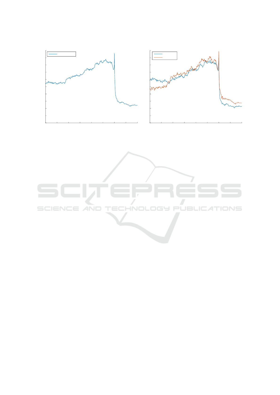
Figure 1: Ratio of ball possession before goal-scoring opportunities for (a) all attacking teams and (b) the featured Bundesliga
team and other teams. t = 0 marks the time of goal-scoring opportunities.
the team whose player was closest to the ball (dis-
tance from ball to closest player had to be below 1.5
meters). Some extra parameters were added to avoid
the algorithm from switching ball possession when
the ball passed a player closely. When the ball did
not undergo a significant change in direction of more
than 20 degrees, or the ball velocity was not under 10
km/h, ball possession was not changed to the nearest
player.
Figure 1 shows ball possession ratios before goal-
scoring opportunities. Figure 1(a) shows possession
before opportunities for the Bundesliga team, while
in figure 1(b) possession before goal-scoring opportu-
nities is compared between the Bundesliga team and
opposing teams. The peak of 1.0 at the moment of
opportunities is the result of the pre-condition of ball
possession for the attacking team for goal-scoring op-
portunities.
2.2.3 Constructing Data for Training and
Testing
Given a specific combination of player and ball posi-
tions, we would like to estimate the probability that
a goal-scoring opportunity will emerge within a rea-
sonable amount of time. This estimation will be done
by classifying examples into two categories: a cate-
gory containing soccer snapshots before goal-scoring
opportunities, and a category containing examples of
the opposite scenario, namely loss of ball possession.
It can be quite a challenge to classify a specific sit-
uation on the pitch into one of the above categories.
This challenge becomes even harder when the win-
dow around goal-scoring opportunities is enlarged:
when not only the exact instant of the shot on goal
is considered a goal-scoring opportunity, but also the
5 or 10 seconds before the event. While more of
a challenge, a bigger window is beneficial for the
predictive power of the classifier as it obtains more
positive examples. It enables more practical uses as
well: with an extended window, one could possibly
use the classifier for predicting goal-scoring oppor-
tunities in the next couple of seconds. For the cur-
rent research, a goal-scoring opportunity window of
10 seconds has been used. Explicitly, this means that
samples extracted from the 10-second interval before
goal-scoring opportunities were considered instances
of the opportunity class. The same applied to the loss
of ball possession class: samples from the 10-second
interval before loss of ball possession were still con-
sidered class instances. Not all instances of ball pos-
session loss were extracted and fed to the classifiers:
the ball had to be lost on the attacking side of the field
with respect to the considered team.
As input to the machine learning algorithms,
256 × 256 RGB color images were used. Images are
suitable for visualizing player positions because the
dataset consists of two-dimensional coordinates of the
objects on the field: the height of the objects was not
captured. The players and ball can therefore be rep-
resented by blobs on the images, such as rectangles
and circles. For every detected event (opportunity or
loss of ball possession), samples were taken from the
10-second interval before the event with a spacing of
1 second. For all images, mirrored versions with re-
spect to the x-axis were added to the dataset as well.
Figure 3 depicts sample images which were used
for learning. Both images were constructed from po-
ICPRAM 2017 - 6th International Conference on Pattern Recognition Applications and Methods
450
(a) (b) (c) (d)
(e) (f) (g) (h)
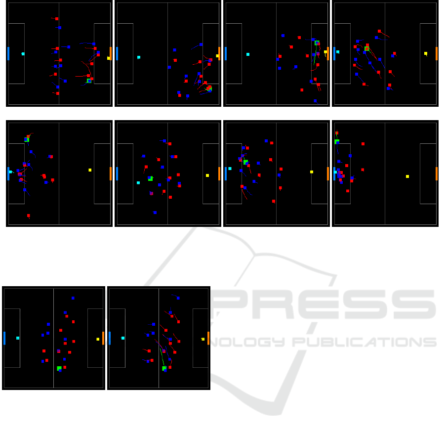
Figure 2: 8 enhanced images extracted from the intervals before different match events. The top row images (a-d) belong to
the positive, opportunity class; the bottom row images (e-h) to the negative, loss of ball possession class. Note that mirrored
images around the x-axis are used as well in the dataset.
(a) Original (b) Enhanced
Figure 3: Example of images used as input for the con-
volutional neural networks. Both images depict the same
moment in time, but the enhanced images also show object
trajectories for the last 2 seconds.
sition data from the same time step. The left image
was constructed solely by looking at the current sam-
ple, while the right image incorporates information
from previous samples as well. The trail behind ob-
jects shows the past positions for the 2 seconds before
the captured moment. The convolutional neural net-
works were trained independently with original and
enhanced images, and were compared in terms of ac-
curacy.
To illustrate how samples belonging to the dif-
ferent classes were transformed to images, figure 2
shows 4 randomly selected positive examples and 4
randomly selected negative examples. The top row
images (a-d) belong to the positive, or goal-scoring
opportunity, class. Within 10 seconds of the de-
picted scenarios, goal-scoring opportunities were cre-
ated. The same applies to the bottom row images (e-h)
which show negative examples. Within 10 seconds of
the shown scenarios, ball possession was lost by the
attacking team.
To facilitate learning, the same Bundesliga team
was always playing from right to left on the images,
and marked as red (players) and yellow squares (goal-
keeper). The opposing team’s players’ positions were
displayed as blue (players) and light blue (goalkeeper)
squares. The size of the squares for players was
7 × 7 pixels, while the green colored ball was of size
11 × 11 pixels. The ball was always printed on the
background. When two players’ positions did par-
tially overlap, the colors of these players were mixed,
resulting in a purple color for a red and blue player.
Some experiments were done for varying sizes of
squares, but this did not affect the performance of the
classifiers much. Therefore the size for the players
and ball was kept as small as possible for maximum
detail.
3 METHODS
Convolutional Neural Networks (CNNs) are a type
of neural networks which excessively make use of
mathematical convolutions to learn a function which
Using Deep Convolutional Neural Networks to Predict Goal-scoring Opportunities in Soccer
451
is non-linear in nature. CNNs are particularly suited
for image data because of convolution kernels which
are shifted over an image. A fully-connected multi-
layered perceptron would be overly connected to the
input image and therefore focus too much on single
pixels instead of patterns spanning multiple pixels.
The first CNN which appeared in literature in
1990 (LeCun et al., 1990) used a small neural net-
work incorporating two convolutional layers to rec-
ognize handwritten digits. Over the last few years,
CNNs and deep learning have experienced an enor-
mous boost in popularity. This can mainly be ascribed
to their recent successes in the Imagenet Large Scale
Visual Recognition Challenge (ILSVRC) (Deng et al.,
2009). The following subsections are used to describe
the methods used to carry out our experiments.
3.1 GoogLeNet
For the current research, GoogLeNet was selected
as the most complex CNN to function in our exper-
iments. Opposed to ILSVRC2012 winner AlexNet
(Krizhevsky et al., 2012), which used relatively few
convolution kernels which acted on big volumes
of data, GoogLeNet introduced so-called Inception
modules. In an Inception module convolutions with
differently sized kernels are applied in parallel. The
outputs of the multiple convolutional layers within a
module are concatenated and passed to the next layer.
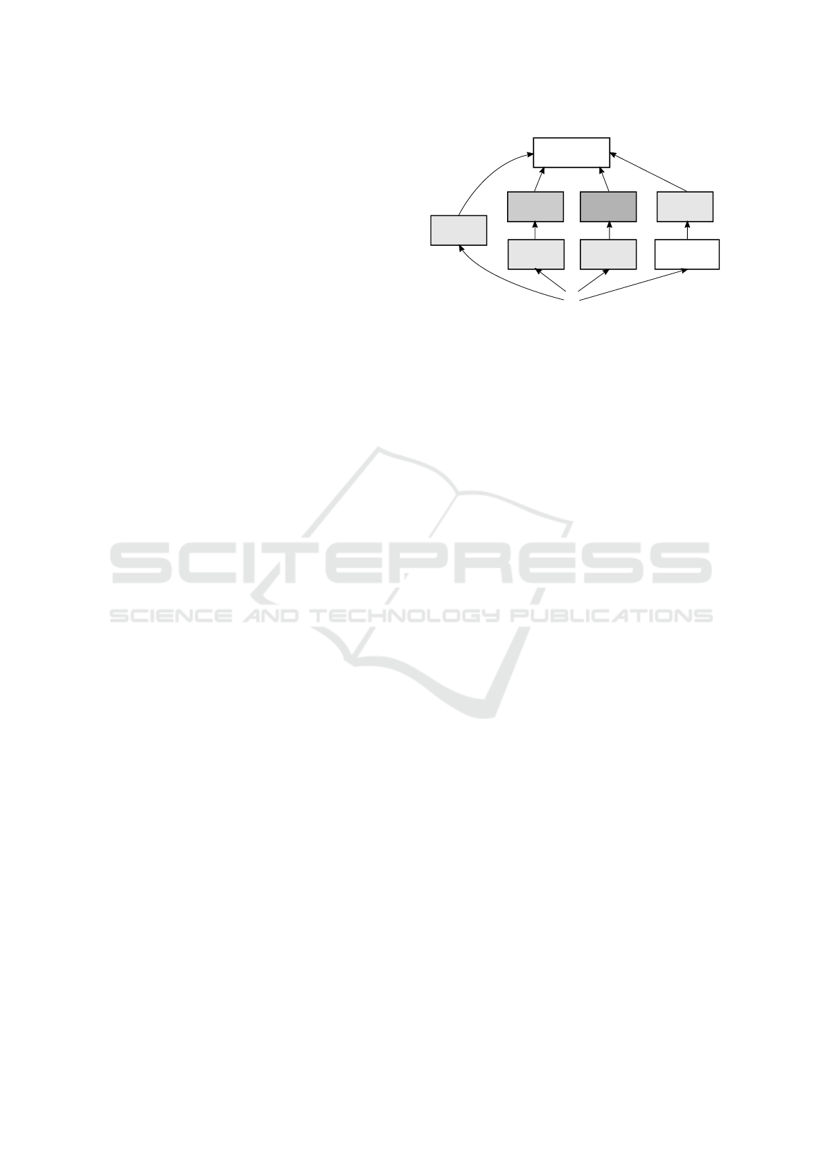
Figure 4 shows an illustration of a single Inception
module. In the full CNN, Inception modules were
stacked on top of each other, where the output of the
previous module functioned as the input for the next.
Deep convolutional neural networks have the un-
desired property that the volumes of data, due to re-
peated convolutions, quickly become too large to be
handled by current computer hardware. Some net-
works attempt to tackle this issue by using subsam-
pling methods such as average or maximum pooling.
In GoogLeNet, every time the computational require-
ments would increase too much to be handled by the
hardware, the dimension of volumes is reduced. This
is achieved both by using max pooling (average pool-
ing in a few cases) and 1 × 1 convolutions. This is
clearly visible in figure 4: before 3 × 3 and 5 × 5 con-
volutions, the input is convolved with small 1 × 1 ker-
nels.
Because GoogLeNet is a very deep network with
22 layers with parameters (excluding pooling lay-
ers which do not have parameters/weights), it can
be hard to correctly adapt the weights using back-
propagation. There is a problem of vanishing gra-
dients: the error vanishes when it is propagated
back into the network, leading to insufficient weight
x
5x5 conv
3x3 conv
1x1 conv 3x3 max pool
1x1 conv
1x1 conv
1x1 conv
Filter
concatenation
Figure 4: A single Inception module. Image based on
(Szegedy et al., 2015).
changes in the neurons near the input (Bengio et al.,
1994). GoogLeNet tackles this problem by adding
two auxiliary classifiers to the network, which are
connected to intermediate layers. The output of these
layers was taken into account for back-propagation
during training: the error of the auxiliary classifiers
was weighted with a factor 0.3 (opposed to 1.0 for the
final, ‘third’ output). In this way, the error did not
vanish as much as it would if there had only been one
output, as the intermediate classifiers were closer to
the input than the final classifier. The auxiliary classi-
fiers were not taken into account during test and vali-
dation time.
GoogLeNet showed spectacular performance on
the Imagenet dataset: a top-5 error of 6.67 was
achieved, which is significantly better than the error
rate of ILSVRC2013 winner Clarifai (11.2) (Zeiler
and Fergus, 2014). Although GoogLeNet achieved
a very good performance on the Imagenet dataset, it
should also be suitable for images constructed from
soccer data. There might be too many layers be-
cause of our abstract data representation with rela-
tively few features, although the intermediate out-
puts of GoogLeNet should have sufficient measures
to handle this. A GoogLeNet implementation in
Caffe (Jia et al., 2014) was trained both starting from
scratch (with randomized starting model parameters)
and from a pre-trained model (which was distributed
with Caffe and trained on the Imagenet dataset). Be-
cause the Imagenet dataset contained 1000 classes
and in this paper we are dealing with two classes, the
last pre-trained layer from GoogLeNet could not be
re-used, as the network had to use a 2-way softmax
function instead of 1000-way softmax regression.
Training and testing was done with datasets con-
taining only original images and with datasets con-
taining enhanced images with added object trails.
This leads to a total of 4 experiments:
1. Experiment 1a: GoogLeNet trained from
scratch, default data.
ICPRAM 2017 - 6th International Conference on Pattern Recognition Applications and Methods
452
2. Experiment 1b: Pre-trained GoogLeNet, default
data.
3. Experiment 1c: GoogLeNet trained from
scratch, enhanced data.
4. Experiment 1d: Pre-trained GoogLeNet, en-
hanced data.
The GoogLeNet models were trained on 6300 im-
ages for 8 epochs with a learning rate of 0.001. The
learning rate was decreased by a factor 10 every 33%
of the epochs (2.67 epochs). The stopping crite-
rion was determined by taking the validation error on
1400 validation images into account. A momentum
of 0.9 was used and a weight decay with λ = 0.0005
(Sutskever et al., 2013; Jacobs, 1988; Moody et al.,
1995). Nesterov’s accelerated gradient was used as a
solver for the network (Nesterov, 1983), which is a
variant of stochastic gradient descent with the differ-
ence that the gradient is taken on the current weights
with added momentum, as opposed to stochastic gra-
dient descent which only takes the current weights
into account for computing the gradient. The mini-
batch size for training was set to 8. The neural net-
works were tested on datasets containing 6300 im-
ages, leading to a train-validation-test distribution of
45%-10%-45%. All sets consist of exactly 50% im-
ages from the positive class and 50% images from the
negative class.
3.2 3-Layered Convolutional Neural
Network
The performance of GoogLeNet was compared to a
straightforward, self-constructed convolutional neu-
ral network with 3 convolutional layers. Convolu-
tions were computed sequentially on big volumes of
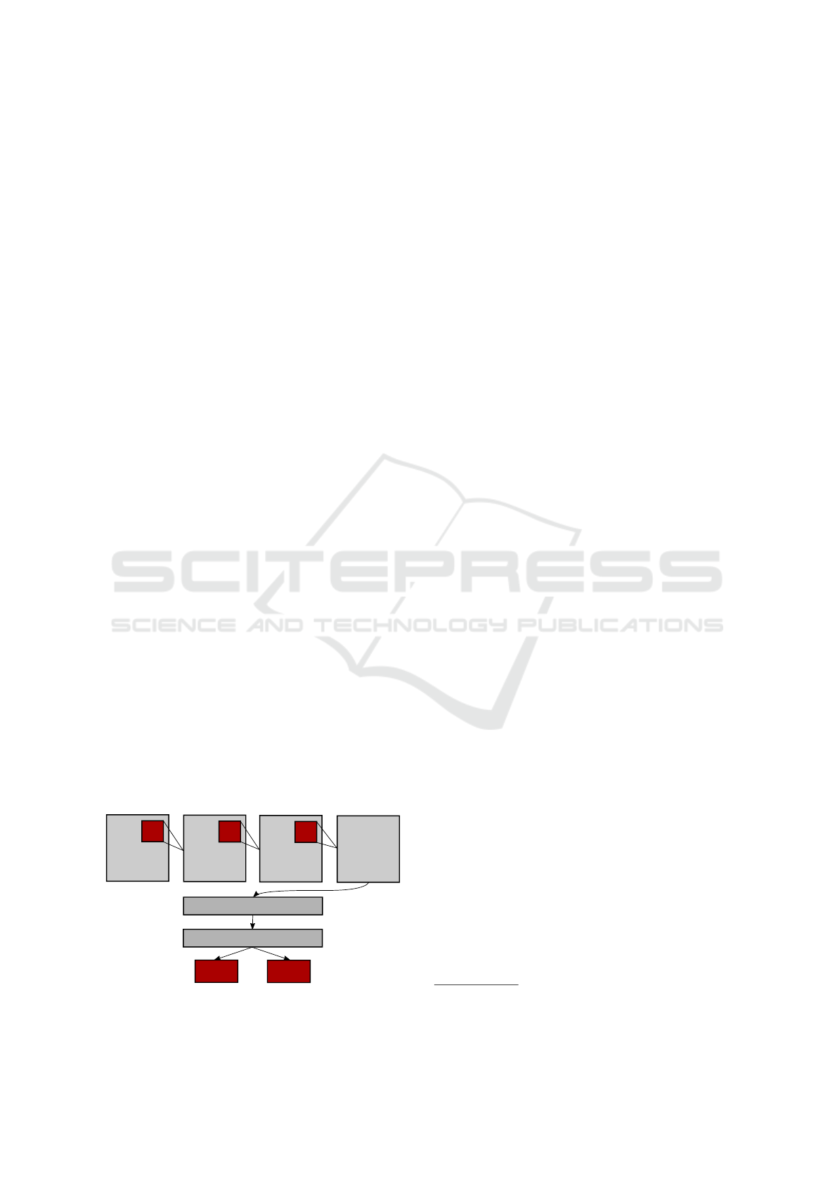
intermediate data. Figure 5 shows the structure of this
CNN architecture.
The first convolutional layer takes the input and
convolves it with 48 kernels of size 7 × 7 with a
stride of 2. The number of kernels in this layer
Input image
256x256x3
7x7
Conv1
5x5
Conv2
3x3
Conv3
fc1 (1000 neurons)
fc2 (1000 neurons)
Output
class 1
Output
class 2
48 kernels 128 kernels
192 kernels
Figure 5: The 3-layered convolutional neural network used
for experiment 2.
was intentionally left low because of the very simple
shapes that were used to construct the images in the
datasets. The convolutional layer was followed by a
ReLU unit (Nair and Hinton, 2010) and a max pooling
layer with size 3 × 3 and stride 2 (similar to AlexNet
(Krizhevsky et al., 2012)). The second convolutional
layer consists of 128 kernels of size 5 × 5, and is fol-
lowed by ReLU units and a max pooling layer with
the same hyper-parameters as described previously.
The third and last convolutional layer houses 192 ker-
nels of size 3 × 3 whose output is passed through a
ReLU and max pooling layer.
The 3-layered convolutional neural network was
trained for 2 epochs on every dataset. This stopping
criterion was determined by taking validation set per-
formance into account. The learning rate was set to
0.00005 and decreased with a factor 10 every 33%
of the epochs (0.67 epochs). The datasets used for
training and testing, the solver method and values
for weight decay and momentum were equal to those
used for GoogLeNet.
For the smaller CNN, two experiments were con-
ducted: one with the original data, and another with
enhanced data.
1. Experiment 2a: 3-layered CNN with default
data.
2. Experiment 2b: 3-layered CNN with enhanced
data.
3.3 KNN Baseline
A final k-nearest neighbors experiment
functioned as a baseline (Cover and Hart,
1967). K-nearest neighbors was trained on
ball positions of 50 percent of a dataset:
(x
ball,1
, y
ball,1
), (x
ball,2
, y
ball,2
), . . . , (x
ball,7000
, y
ball,7000
).
For testing, the other half of the data was sequentially
presented. To every testing example (x
ball,n
, y
ball,n
),
the class of the majority of the k = 25 nearest training
examples was assigned
1
. The euclidean distance
was used as distance measure. The accuracy was
then calculated by dividing the number of correctly
classified examples by the total number of test
examples. For KNN, 7000 training images and 7000
test images were used per dataset division.
Experiment 3. K-nearest neighbor classification
1
Multiple values of k were tested. The best results were
achieved with k = 25.
Using Deep Convolutional Neural Networks to Predict Goal-scoring Opportunities in Soccer
453
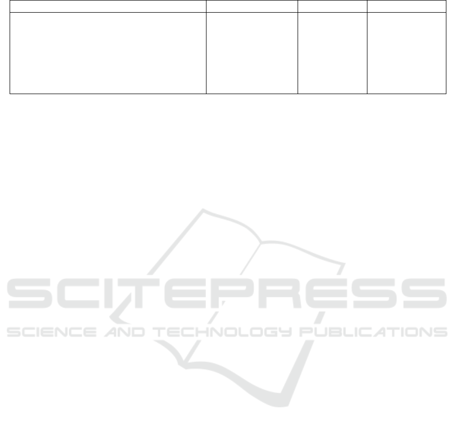
Table 1: Average classification accuracies and standard deviations for all experiments.
Experiment Nesterov (10 runs) SGD (5 runs) Other (10 runs)
1a: GoogLeNet scratch, original images 64.8 ± 2.4% 64.5 ± 2.8%
1b: GoogLeNet pre-trained, original images 63.3 ± 3.0% 62.6 ± 2.3%
1c: GoogLeNet scratch, enhanced images 67.1 ± 2.7% 67.0 ± 3.0%
1d: GoogLeNet pre-trained, enhanced images 65.4 ± 2.3% 66.0 ± 2.6%
2a: 3-layered net, original images 62.4 ± 2.1%
2b: 3-layered net, enhanced images 62.8 ± 1.7%
3: K-nearest neighbors 57.3 ± 1.2%
4 RESULTS AND DISCUSSION
Images belonging to a single opportunity or instance
of ball possession loss were coupled and could not
end up in both training and test sets. Every dataset
split contained samples extracted from all of the 349
detected goal-scoring opportunities. A goal-scoring
opportunity was assigned to either the train, valida-
tion or test set: two arbitrary samples extracted from
a given opportunity always ended up in the same set.
The negative examples (loss of ball possession)
were selected in order to resemble the positive exam-
ples (goal-scoring opportunities) as close as possible.
For every goal-scoring opportunity, an instance of ball
possession loss was selected for the team which cre-
ated the opportunity. This loss of ball possession had
to occur in the same match half as where the coupled
goal-scoring opportunity arose, and on the attacking
half of the field with respect to the considered team.
4.1 Results
In our preliminary experiments, we used the
GoogLeNet architecture with the Nesterov solver to
train the network. The obtained results were good
but there was a need to investigate another solver
type, such stochastic gradient descent (SGD). After 5-
fold random cross-validation, the results did not differ
much from the Nesterov solver experiments. The re-
sults for both the Nesterov solver and SGD are shown
in table 1. The table also shows the performance of
the 3-layered CNN (trained with the Nesterov solver)
and KNN.
GoogLeNet trained from scratch with enhanced
images (experiment 1c) performed best and achieved
an accuracy of 67.1%. This is almost 10 percent
higher than the outcome of the k-nearest neighbors
baseline experiment (accuracy: 57.3%, experiment
3). The 3-layered net performed better than KNN as
well and achieved a top accuracy of 62.8%.
4.2 Discussion
The most complex network used in the experiments,
GoogLeNet, showed top performance with an accu-
racy of 67.1%. Zooming in on the training process of
the GoogLeNet models, the training error was greatly
reduced during the first epoch and did not decrease
much from epoch 2 to 8. The same applied to the
validation accuracy. The reason why training was run
for 8 epochs instead of 2 was that in some cases the
validation accuracy was very low in the beginning,
possibly due to unlucky initialization or an unfavored
sequence of presented inputs, so it did need more it-
erations to achieve a higher level of performance.
The same phenomenon of early convergence of
model parameters was visible for the less complex 3-
layered convolutional neural network. This network
only showed a drop in training error at the very be-
ginning and did not decrease much afterwards. The
accuracy did not improve when it was trained for
more than 2 epochs. It is therefore hard to believe
that the network successfully accomplished to learn
all higher-order patterns of soccer which are impor-
tant for creating opportunities. The network did prob-
ably only manage to learn a set of basic rules, which
led to an average accuracy of a little less than 63%.
The difference in performance and training be-
tween GoogLeNet and the 3-layered convolutional
neural network is interesting. The top-performing
variant of GoogLeNet (trained from scratch, en-
hanced images) achieved an accuracy more than 4%
higher than the 3-layered net, which is a significant
difference. It seems that GoogLeNet is able to capture
more complex tactical patterns than the other models.
The average accuracy increase of approximately
2% for enhanced images over default images is
promising as well. The added information in the
form of object trails seems to be picked up by the
models which use it to their advantage. The images
could possibly be enriched with even more bells and
whistles, which might be interesting to research in
the future. The absence of this difference for the 3-
ICPRAM 2017 - 6th International Conference on Pattern Recognition Applications and Methods
454

layered network suggests that GoogLeNet is indeed
able to catch some higher-order patterns, in which the
3-layered net does not succeed.
Then remains the question how bad an accuracy
of 67.1% actually is. As a starting point, it is signifi-
cantly higher than the 57.3% accuracy of the k-nearest
neighbors baseline. But what would the performance
of the best performing human or artificial classifier
be for the current problem? Would an accuracy of,
say, 90% be realistic? This would probably not be the
case. Samples were extracted already 10 seconds be-
fore the occurrence of goal-scoring opportunities. A
lot can happen in the 10 second interval to the actual
shot towards the goal.
5 CONCLUSION
To conclude, the results suggest that convolutional
neural networks are capable of predicting goal-
scoring opportunities to a certain extent. There are
a couple of ways how the performance of the convo-
lutional neural networks could be improved. Using a
larger dataset would probably stimulate the convolu-
tional neural networks to learn higher-order patterns
instead of more superficial ones. A higher number of
classes can be used to detect more events in soccer,
or input images can be weighted differently by taking
their temporal location to events into account. As an
alternative to using point images, a graph representa-
tion of the position data could be used as input to neu-
ral networks. Finally, using a more specialized con-
volutional neural network, possibly combined with
a recurrent neural network architecture, could yield
higher accuracies, as would using an ensemble of sev-
eral classifiers.
REFERENCES
Barris, S. and Button, C. (2008). A review of vision-
based motion analysis in sport. Sports Medicine,
38(12):1025–1043.
Bengio, Y., Simard, P., and Frasconi, P. (1994). Learning
long-term dependencies with gradient descent is diffi-
cult. IEEE transactions on neural networks, 5(2):157–
166.
Brooks, J., Kerr, M., and Guttag, J. (2016). Using machine
learning to draw inferences from pass location data
in soccer. Statistical Analysis and Data Mining: The
ASA Data Science Journal, 9(5):338–349.
Cover, T. and Hart, P. (1967). Nearest neighbor pattern clas-
sification. IEEE transactions on information theory,
13(1):21–27.
Deng, J., Dong, W., Socher, R., Li, L.-J., Li, K., and Fei-Fei,
L. (2009). Imagenet: A large-scale hierarchical image
database. In Computer Vision and Pattern Recogni-
tion, 2009. CVPR 2009. IEEE Conference on, pages
248–255.
Grunz, A., Memmert, D., and Perl, J. (2012). Tactical pat-
tern recognition in soccer games by means of spe-
cial self-organizing maps. Human movement science,
31(2):334–343.
Jacobs, R. A. (1988). Increased rates of convergence
through learning rate adaptation. Neural networks,
1(4):295–307.
Jia, Y., Shelhamer, E., Donahue, J., Karayev, S., Long, J.,
Girshick, R., Guadarrama, S., and Darrell, T. (2014).
Caffe: Convolutional architecture for fast feature em-
bedding. In Proceedings of the 22nd ACM interna-
tional conference on Multimedia, pages 675–678.
Knauf, K., Memmert, D., and Brefeld, U. (2016). Spatio-
temporal convolution kernels. Machine Learning,
102(2):247–273.
Kohonen, T. and Somervuo, P. (1998). Self-organizing
maps of symbol strings. Neurocomputing, 21(1):19–
30.
Krizhevsky, A., Sutskever, I., and Hinton, G. E. (2012). Im-
agenet classification with deep convolutional neural
networks. In Advances in neural information process-
ing systems, pages 1097–1105.
LeCun, Y., Boser, B., Denker, J. S., Henderson, D., Howard,
R. E., Hubbard, W., and Jackel, L. D. (1990). Hand-
written digit recognition with a back-propagation net-
work. In Advances in neural information processing
systems.
Memmert, D., Lemmink, K. A., and Sampaio, J. (2016).
Current approaches to tactical performance analyses
in soccer using position data. Sports Medicine, pages
1–10.
Moody, J., Hanson, S., Krogh, A., and Hertz, J. A. (1995).
A simple weight decay can improve generalization.
Advances in neural information processing systems,
4:950–957.
Nair, V. and Hinton, G. E. (2010). Rectified linear units
improve restricted boltzmann machines. In Proceed-
ings of the 27th International Conference on Machine
Learning (ICML-10), pages 807–814.
Nesterov, Y. (1983). A method of solving a convex pro-
gramming problem with convergence rate o (1/k2). In
Soviet Mathematics Doklady, volume 27, pages 372–
376.
Sutskever, I., Martens, J., Dahl, G. E., and Hinton, G. E.
(2013). On the importance of initialization and mo-
mentum in deep learning. ICML (3), 28:1139–1147.
Szegedy, C., Liu, W., Jia, Y., Sermanet, P., Reed, S.,
Anguelov, D., Erhan, D., Vanhoucke, V., and Rabi-
novich, A. (2015). Going deeper with convolutions.
In Proceedings of the IEEE Conference on Computer
Vision and Pattern Recognition, pages 1–9.
Zeiler, M. D. and Fergus, R. (2014). Visualizing and under-
standing convolutional networks. In European Con-
ference on Computer Vision, pages 818–833. Springer.
Using Deep Convolutional Neural Networks to Predict Goal-scoring Opportunities in Soccer
455
