
Supporting Harvest Planning Decisions in the Tomato Industry
Eduardo A. Alarcón Gerbier
1
, Marcela C. Gonzalez-Araya
2
and Masly M. Rivera Moraga
1
1
Escuela de Ingeniería Industrial, Universidad de Talca, Camino a los Niches km 1, Curicó, Chile
2
Departament of Industrial Engineering, Faculty of Engineering, Universidad de Talca,
Camino a los Niches km 1, Curicó, Chile
Keywords: Scheduling, Logistics, Integer Programming, Tomato Industry, Harvest Planning.
Abstract: Tomato is a raw material that easily deteriorates once harvested and loaded on trucks, losing juice and flesh.
Therefore, the reduction of trucks’ waiting times in the receiving area of a processing plant can allow reducing
tomato waste. In this article, we develop a model that aims to keep a continuous flow of fresh tomato to a
paste processing plant and to decrease trucks’ waiting times in the plant receiving area. The model is used in
a real case of a tomato paste company. The obtained solutions present a better allocation of the harvest shifts,
allowing more uniform truck arrivals to the plant during the day. Therefore, trucks waiting times are reduced,
decreasing raw material deterioration.
1 INTRODUCTION
The problem of trucks congestion in tomato
processing plants is discussed, which causes high
trucks’ waiting times and deterioration of the
transported raw material.
This problem is especially relevant in the
competitive tomato industry, where the major world
exporters, as USA and China, with 35% and 13% of
world production, respectively, exert a strong prices
pressure (ODEPA, 2013). In 2012, Chile ranked tenth
in the export of tomato paste, with about 100
thousand tons exported per year. On the other hand,
the main tomato paste consumers markets are located
in Europe, Africa, Asia and Middle East, very far
from Chile. Because of this, Chilean companies are
constantly seeking to increase their productivity and
reduce their production costs.
In the supply chain of tomato paste, the
coordination between harvesting, transportation and
production stages is necessary because of during a
production season the plants work 24 hours. In this
sense, a good coordination allows to obtain a
continuous fresh tomato supply to the plants during
the day, reducing trucks’ waiting times and avoiding
fresh tomato deterioration. Therefore, the
productivity of raw material conversion is increased
and so, the production and transportation costs are
diminished.
Many researchers have addressed the supply chain
planning and coordination of agrifood produce.
Ahumada and Villalobos (2009), Díaz-Madroñero et
al. (2015) and Soto-Silva et al. (2016) present reviews
of optimization models that support decisions in
different stages of the supply chain, and for different
kind of agricultural products.
Related to harvest planning coordination, in the
literature is possible to found a considerable number
of articles devoted to the sugarcane industry (Higgins,
2006, López-Milán, and Plà-Aragonés, 2015,
Pathumnakul and Nakrachata-Amon, 2015, Lamsal et
al., 2015, Lamsal et al., 2016, among others).
However, these models are usually specific to each
country and industry, because of differing levels and
different infrastructures of vertical integration, as
specified by Lamsal et al. (2016).
In their work, Higgins (2006) and Lamsal et al.
(2015, 2016) present optimization models that aim to
reduce trucks’ waiting times.
Higgins (2006) presents a mixed integer
programming model, which deals with the trucks
congestion problem in the sugar mills of Australia.
The model seeks to minimize the trucks’ queue time
and the sum of the mills’ idle time. This model has a
high complexity, because of it also incorporates the
generated queue in each each mill. For this reason,
Variable Neighborhood Search (VNS) and Tabu
Search algorithms are developed to solve it.
A. Alarcøsn Gerbier E., C. Gonzalez-Araya M. and M. Rivera Moraga M.
Supporting Harvest Planning Decisions in the Tomato Industry.
DOI: 10.5220/0006193203530359
In Proceedings of the 6th International Conference on Operations Research and Enterprise Systems (ICORES 2017), pages 353-359
ISBN: 978-989-758-218-9
Copyright
c
2017 by SCITEPRESS – Science and Technology Publications, Lda. All rights reserved
353

Lamsal et al. (2015) propose an integer
programming model that seeks to coordinate the
harvest and transport of sugarcane supply chain in
order to reduce trucks waiting times. For achieving
this goal, the proposed model maximizes the
minimum gap between two successive arrivals in a
sugar mill.
Lamsal et al. (2016) propose a model to plan
trucks movement between harvest and plants. This
model is applicable when there are multiple and
independent producers and it is not convenient to
store fresh produce in the place of the harvest. The
methodology used by these authors is divided in two
stages. In the first stage, a model to determine the
harvest start times is run. In the second stage, an
algorithm for determining the number of trucks to
transport raw materials is executed.
In this research is applied a version of the model
developed by Lamsal et al. (2016), using data from a
Chilean company. The company requires a tool for
supporting decision to determine start times of tomato
harvesting machines and the number of trucks to
assign in each farm, every day. In this way, the
company can guarantee a continuous flow of raw
materials to the plants and to reduce trucks’ waiting
times and the tomato deterioration.
Therefore, this paper is structured as follows. In
Section 2, the description of transport and harvest
problem is presented. In Section 3, the proposed
mathematical model for determining daily harvest
start times of each tomato farm is explained and, in
Section 4, a case study of the tomato paste company
is carried out. Finally, in Section 5 the conclusions as
further research are presented.
2 HARVEST PLANNING AND
TRANSPORT TO A TOMATO
PROCESSING PLANT
In agribusiness, companies generally ensure their
plants’ supplies by purchasing fresh raw materials
from different suppliers, located in areas as near as
possible to the plants. For this reason, before the
harvest season, the companies make contracts to
purchase all the yield of the suppliers’ farms. This
behaviour is also observed in the tomato industry.
In the harvest season, the tomato harvesting
machines are outsourced and they move to each farm
according to the harvest plan established by the
company.
As the tomato harvesting activities, the fresh raw
material transport from the harvest sites to the
processing plants is also outsourced.
Every day, the selection of tomato farms to be
harvested is performed according to the information
about tomato ripening in each field and the daily
demand of each plant. The trucks allocation to the
farms depend on each transport contractor, which has
assigned one or more harvesting machines. The
contractor is responsible for determining which truck
will transport fresh tomato to a plant, based on the
number of daily truckload per harvesting machine
estimated by the company. In general, it does not exist
a decision support system for carrying out this
activity.
Each company determines the working hours of
tomato harvesting machines, but it is very common
that companies have fixed shifts during the day. Most
harvesting machines are used during the morning and
the afternoon that involves high trucks demand in
these periods.
Once a truck arrives to the receiving area of a
plant, a download code is assigned to it.
Subsequently, it is weighed and recorded at the
gathering place, where trucks wait their shift to the
next stage. Once the plant requires its fresh raw
material, the truck goes to the quality control process,
where the percentage of damage is determined based
on a sample of 20 kilograms. Finally, the truck is
directed to a defined placement area where it
proceeds to unload the tomato.
The plants operate 24 hours every day, therefore,
they require a continuous flow of raw material and,
consequently, a continuous flow of trucks. However,
because of work shifts established for the farms are
mainly concentrated during the morning and the
afternoon, the truck arrivals to the receiving area of
the plants are concentrated from the afternoon. This
situation causes trucks congestion, so each truck
waits in the receiving area on average four hours. This
problem involves an increase of transportation costs
due to the number of hours spent by trucks in the
receiving area and implies a tomato deterioration
during waiting time, because of juice and flesh loss.
In Table 1, the effect of waiting times decrease for
a constant level of production is shown. It is possible
to observe that a decrease in one hour of waiting
times, for a same level of production, reduces in 85.4
tons the plant raw material requirements. These data
were obtained from a Chilean company that
manufactures tomato paste.
ICORES 2017 - 6th International Conference on Operations Research and Enterprise Systems
354

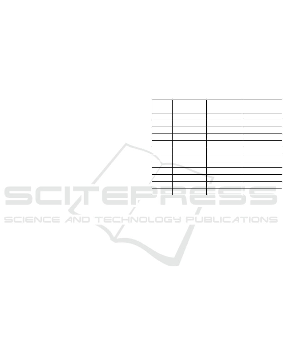
Table 1: Effect of waiting times in tomato deterioration.
Decrease in
the waiting
time (hour)
No. kg tomato
per kg tomato
paste
No. ton
of
tomatoes
Daily
savings
(ton)
0:30
5,42 3.004,6 40,8
1:00 5,34 2.960,0 85,4
1:30 5,25 2.912,5 132,9
2:00 5,16 2.861,7 183,7
2:30 5,06 2.807,8 237,6
In this sense, in order to improve the supply
efficiency, the development of a model to plan
operations for both, harvest and transport activities, is
necessary, aiming to obtain a constant flow of trucks
during the day, to decrease the trucks waiting times at
the receiving area of plants and so, to reduce raw
material deterioration.
3 MODEL FOR HARVEST
PLANNING
The following sets are used in the model:
C
i
: set of loads at farm i, i ∈ I, j ∈C
i
.
I: set of farms to be harvested.
The parameters considered by the model are the
following:
n: number of blocks of time in which the day is
divided.
a
: start time of the block k, for k= 0, 1, …, n.
Furthermore a
<a
<a
…<a
, where a
represents the end time of the delivery window.
h
i
: time required to harvest a load at farm i, i ∈ I.
N
k
: unloading capacity in the plant for each block
k=0, 1, …, n-1.
t
i
: travel time between farm i and the plant, i ∈ I.
α: penalization associated with the deviation of the
plant’s unloading capacity.
lmt: maximum number of farms that can be harvested
in shift 3.
The decision variables of the model are the
following:
x
: arrival time at the plant of ith farm’s jth load, i ∈
I y j ∈ C
i
.
y
: time when the harvesting starts at farm I, i ∈ I.
: ∈ R+ and expresses the instant in which the jth
load of the ith farm lies between the time a
and
a
, i ∈ I, j ∈ Ci and k= 0, 1, …, n.
: ∈ {0,1}, where
= 1 if the ith farm’s jth load
arrives between a
and a
,
= 0 otherwise.
: surplus capacity or positive deviation from the
plant’s unloading capacity, k= 0, 1, …, n-1.
: slack capacity or negative deviation from the
plant’s unloading capacity, k= 0, 1, …, n-1.
: ∈ {0,1}, where
= 1 if the shift 3 is
available to be assigned in the farm i,
= 0
otherwise.
The formulation of the proposed model for
harvest planning is presented in this section. The
indices, parameters and decision variables of the
model can be founded in the Appendix.
Mathematical formulation
MinZ
α∗CF
1α
∗CS
(1)
s.t.
x
y
j∗h
t
∀i∈I,j∈C
(2)
x
λ
∗a
∀i∈I,j∈C
(3)
λ
1 ∀i ∈ I,j∈C
(4)
λ
b
∀i ∈ I,j∈C
(5)
λ
b
b
∀i∈I,j∈C
,
k∈1,…,n
(6)
b
0 ∀i ∈I,j∈C
(7)
b
1 ∀i ∈I,j∈C
(8)
b
∈
∈
CS
CF
N
∀k
∈0,…,n1
(9)
b
Є0,1 ∀i ∈I,j∈C
,k∈0,…,n
(10)
λ
Є0,1 ∀i ∈I,j∈C
,k∈0,…,n
(11)
CF
,CS
0 ∀k∈0,…,n1 (12)
y
0 ∀i ∈I
(13)
x
0 ∀i ∈I,j∈C
(14)
Supporting Harvest Planning Decisions in the Tomato Industry
355
The objective function minimizes positive and
negative deviation from the plant’s unloading
capacity. Depending on the case can be penalized just
one of the deviation or more heavily in one direction
than the deviation on the other side. For example, to
achieve a high utilization of the plant should be
penalized the slack capacity (CF
) and to minimize
the downtime of the trucks should be penalized
specially the surplus capacity (CS
).
Constraint (2) states that the arrival time at the
plant of ith farm’s jth load depends on the harvest start
time in the farm i, the harvest rate at that farm and the
travel time between the farm and the plant. Constraint
(3) – (8) determine the arrival time through a convex
combination of the beginning and the end time of
each block into which the arrival falls.
Constraint (9) determines the slack or surplus
capacity in each block by comparing the quantity of
inputs with the unloading capacity.
Finally, the constraints (10) – (14) stablish the
nature of the decision variables.
4 CASE STUDY
In this section the model is used in a real case, which
is based on data from a tomato paste company.
This company has two production plants, where
annually 550,000 tons of fresh tomato are processed.
The raw material is purchased from different farmers
and it is daily harvested using 40 tomato harvesting
machines. These harvesters are mostly subcontracted
and assigned to the farms according to the percentage
of tomato ready to be harvested in each one (from
90% of ripe tomato). For this assignment is used a
manual scheduling.
The company works with three work shifts, which
start at 07:00, 13:00 and 17:00 hours; shifts 1, 2 and
3, respectively. In addition, its plants operate 24 hours
a day. In order that the model assigns to the harvesting
machines these times, the function (15) is established.
It is important to mention that 7 hours are subtracted
from the schedules with the aim of working with
values between 0-24.
0:00
6:00
10:00∗
∀i∈I
(15)
At the same time, because it is difficult to harvest
at night (shift 3), a binary variable (MX
i
) and
restriction (16) is defined. Thus, the total number of
shifts 3 assigned to the harvesters is restricted.
∈
∀i∈I
(16)
4.1 Dataset
To implement the model are used data of harvest from
the season 2016 for one of the plants of the company.
This plant is normally supplied for 12 farms.
Table 2 shows the data of the farms that supply
the plant.
Table 2: Number of loads, travel time and harvest time from
the farms that supply the plant.
Farm Number of
loads
Harvest
time (hour)
Travel time
(hour)
#1 9 1,1 1,6
#2 6 1,7 0,8
#3 10 1,0 0,3
#4 4 2,5 0,6
#5 3 3,3 1,5
#6 7 1,4 0,6
#7 8 1,3 0,3
#8 6 1,7 0,9
#9 6 1,7 1,1
#10 5 2,0 0,3
#11 9 1,1 0,3
#12 10 1,0 0,8
The case study was performed on an 2,40 GHz
Intel Core i3 CPU running the Windows 10 operating
system. The computational results associated to the
case study are obtained using IBM ILOG CPLEX
Optimization Studio version 12.6.
Three scenarios are solved, since the maximum
number of work shifts 3 to be allocated is modified.
The first run (case 1) uses the same proportion of
harvesting machines in each shift that the company
assigned on that day for the farms. With this, the goal
is to determine the optimal distribution while
maintaining the number of harvesting machines
working on each shift. In the second run (case 2) is
limited to a maximum of 25% of the farms to be
harvested on shift 3. This equates to a maximum of
three farms. Finally, in the third run (case 3) the
amount of farms that can be harvested in shift 3 is not
limited.
For all instances, the software takes less than 1
minute. It is noteworthy that, since it is a daily
planning, are needed low runtimes software.
ICORES 2017 - 6th International Conference on Operations Research and Enterprise Systems
356
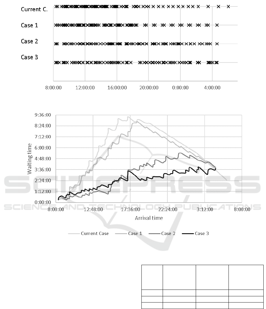
Figure 1: Distribution of arrivals during the day.
Figure 2: Waiting times per hour for each case.
4.2 Main Results
Table 3 compares the real shifts assigned to the farms
with those obtained by the model. It can be seen that
in the real distribution of harvesters (real allocation
and case 1), the schedule most commonly used is the
shift 1. On the other hand, the schedules for
unrestricted modelled case (case 3) are spread more
evenly between shift 1 and shift 3. This is based on
that, a more even distribution of shifts during the day,
allows more uniformity in the arrival of trucks and,
consequently, of load and raw materials. Regarding
the case with restriction (case 2), similar results are
obtained to the real distribution (case 1). However,
greater use of shift 2 and shift 3 is observed.
Table 3: Results for each case.
Shift Real
allocation
and Case 1
Limited
allocation
in shift 3
(Case 2)
No limited
allocation in
shift 3 (Case
3)
#1 10 6 5
#2 1 3 1
#3 1 3 6
Figure 1 shows arrivals of trucks to the plant for
each case. It can be seen that for the real case the most
trucks arrive at the plant during 8:00 and 16:00 hours.
For case 1, which considers the same proportion of
harvesting machines in each shift that the real
allocation, is observed a high arrival rate until about
19:00 hours. The allocation of work shifts, which are
obtained for the optimization model for case 2,
Supporting Harvest Planning Decisions in the Tomato Industry
357

generate a more uniform distribution during the day
compared to the two previous cases. Finally, arrivals
associated to case 3 present a high uniformity.
In order to analyse the impact of the model
solutions in improving the planning of harvest shifts,
software Arena Simulation, version 14.7 is used to
perform this analysis. The simulation allows to
calculate waiting times and queues generated on the
plants in each case.
Figure 2 shows waiting times of the trucks in plant
in relation to its arrival time. The graph shows a
significant decrease in waiting times for cases 2 and
3, compared to cases 1. It is important to note that, for
example, the trucks arriving at 18:00 hours, based on
the allocation of real case and case 1, must wait about
8 hours in the plant for the download process. With
respect to cases 2 and 3, waiting times decrease
considerably, obtaining a waiting on plant close to 3
hours at 18:00 hours.
Table 4 shows the average and maximum waiting
times, as well as the number of trucks in queue for
each case.
For case 1 are obtained average waiting times 4:51
hours, which represents a decrease of about 30
minutes compared to the real case. With respect to
case 2 and case 3 it is obtained a considerable
reduction in waiting times for trucks on plant
compared to real case and case 1, yielding an average
of 2:53 hours for case 2 and 2:22 hours case 3. With
respect to the number of trucks that are in plant for
the download process is obtained on average 8.5
trucks for case 2 and 6.9 trucks for case 3.
The implementation of the model in case 3 causes
a decrease in waiting times of up to 3 hours compared
to the real case. At the same time, the schedules that
consider restrictions on the amount of farm that can
be harvested in shift 3 (case 2) provide equally better
results than manual planning. It is important to
emphasize that the scenarios with constraints on shift
3 are more likely to implement in the operations of
the company, since working during night hours is
more dangerous because of the lack of light and
because the night shifts are more difficult to manage
and control.
Based on these results, it is possible to conclude
that the use of the model allows to obtain a better
allocation of the harvest shifts, which allows truck
arrivals more uniform during the day and, therefore,
shorter waiting times and a decrease in the
deterioration of the raw material.
Table 4: Waiting times and trucks queued for each case,
according to the simulation.
Wait time
(hour)
Number of
trucks in queue
Current
case
Average 5:22:00 16,2
Maximum 9:23:12 33
Case 1 Average 4:51:42 13,2
Maximum 8:54:14 26
Case 2 Average 2:53:35 8,5
Maximum 5:23:33 18
Case 3 Average 2:22:47 6,9
Maximum 3:52:55 13
5 CONCLUSIONS
The optimization model was used in a real case of a
tomato paste company. In this application, three cases
were analyzed. The first case use the same shifts’
distribution established by the company (case 1). The
second case allows only to allocate a maximum of
25% of the farms in the shift 3 (case 2). Finally, the
last case does not limit the allocation of the farms in
every shift (case 3).
The use of the model allows obtaining better shift
allocation of harvesting machines, which improves
the arrival distribution of trucks into the plants. The
case 3, that does not limit the number of farms
assigned to shift 3, presents the best harvesting
machines allocation, which helps to reduce the
trucks’ waiting times in about three hours. However,
this allocation is difficult to implement in any
agribusiness company, because it requires that many
farms be allocated in the evening or night shift (shift
3). In general, workers do not like be assigned at the
last shift. Additionally, night shifts are difficult to
manage and control.
For the other hand, the company can implement
more easily the obtained solutions for cases 1 and 2.
The model solution for case 1 distributes in a better
way than the current situation, the farms and
harvesting machines allocated in each shift. The
solution for case 2, that allows an increase up to 25
percent of farms assigned to shift 3, is more feasible
to be implemented by the company and shows a
decrease of about 2:30 hours of trucks’ waiting time.
According to these results, the impact of solutions
implementation in the company could be high. If a
decrease of about 2:30 hours of trucks’ waiting time
takes place, based on the data presented in Table 1,
saving of around 237.6 tons of tomato could be
obtained. Similarly, the obtained solution in case 1
could allow savings of 40.8 tons per day. In addition,
ICORES 2017 - 6th International Conference on Operations Research and Enterprise Systems
358

reducing trucks waiting times in the plant could speed
up the tomato supply and help to reduce the number
of trucks required for transportation, causing a
decrease of transportation costs.
The use of the model for assigning harvest shifts
obtain better and faster results than the current
allocation method utilized by the company.
Moreover, the model execution requires little
computational time for obtaining solutions, which is
a necessary condition for a daily planning. For
implementing the model, a following stage is to
develop decision support system, so users could
interact easily with the model entering data and
parameters, and getting suitable harvest plan reports.
For future extensions of the model, it could be
interesting to plan harvest activities for a longer
period, as for example a week. This dynamic model
could include the reduction of harvesting machines’
shift changes that are not considered when a daily
plan is executed. Furthermore, this new model
extension could also minimize harvesting machines
displacement during the period.
REFERENCES
Ahumada, O., & Villalobos, J. R. (2009). Application of
planning models in the agrifood supply chain: A
review. European Journal of Operational Research,
196(1), 1–20.
Díaz-Madroñero, M., Peidro, David & Mula, Josefa (2015).
A review of tactical optimization models for integrated
production and transport routing planning decisions.
Computer & Industrial Engineering, 88(10), 518–535.
Higgins, A. (2006). Scheduling of road vehicles in
sugarcane transport: A case study at an Australian sugar
mill. European Journal of Operation Research. 170(3),
987–1000.
Lamsal, K., Jones, P. C. & Thomas, B. W. (2016). Harvest
logistics in agricultural systems with multiple,
independent producers and no on-farm storage.
Computer & Industrial Engineering, 91(1), 129–138.
Lamsal, K., Jones, P. C. & Thomas, B. W. (2015).
Continuous time scheduling for sugarcane harvest
logistics in Louisiana. Computer & Industrial
Engineering, 54(2), 616–627.
López-Milán, E., Plà-Aragonés, L.M. (2015). Optimization
of the supply chain management of sugarcane in Cuba.
In International Series in Operations Research and
Management Science, 224, 107-127.
ODEPA (2016). La industria de la pasta de tomate (2016),
de Oficina de Estudios y Políticas Agrarias. Avaible
from <www.odepa.gob.cl>.
Pathumnakul, S., Nakrachata-Amon, T. (2015). The
applications of operations research in harvest planning:
A case study of the sugarcane industry in Thailand,
Journal of Japan Industrial Management Association,
65 (4E), 328-333.
Soto-Silva, W. E., Nadal-Roig, E., González-Araya, M. C.,
Pla-Aragones, L. M. (2016). Operational research
models applied to the fresh fruit supply chain.
European Journal of Operation Research, 251(2), 245–
355.
Supporting Harvest Planning Decisions in the Tomato Industry
359
