
Approximate Bayes Optimal Policy Search using Neural Networks
Micha
¨
el Castronovo, Vincent Franc¸ois-Lavet, Rapha
¨
el Fonteneau, Damien Ernst and Adrien Cou
¨
etoux
Montefiore Institute, Universit
´
e de Li
`
ege, Li
`
ege, Belgium
Keywords:
Bayesian Reinforcement Learning, Artificial Neural Networks, Offline Policy Search.
Abstract:
Bayesian Reinforcement Learning (BRL) agents aim to maximise the expected collected rewards obtained
when interacting with an unknown Markov Decision Process (MDP) while using some prior knowledge.
State-of-the-art BRL agents rely on frequent updates of the belief on the MDP, as new observations of the
environment are made. This offers theoretical guarantees to converge to an optimum, but is computationally
intractable, even on small-scale problems. In this paper, we present a method that circumvents this issue by
training a parametric policy able to recommend an action directly from raw observations. Artificial Neural
Networks (ANNs) are used to represent this policy, and are trained on the trajectories sampled from the prior.
The trained model is then used online, and is able to act on the real MDP at a very low computational cost.
Our new algorithm shows strong empirical performance, on a wide range of test problems, and is robust to
inaccuracies of the prior distribution.
1 INTRODUCTION
Bayes-Adaptive Markov Decision Processes
(BAMDP) (Silver, 1963; Martin, 1967) form a
natural framework to deal with sequential decision-
making problems when some of the information is
hidden. In these problems, an agent navigates in
an initially unknown environment and receives a
numerical reward according to its actions. However,
actions that yield the highest instant reward and
actions that maximise the gathering of knowledge
about the environment are often different. The
BAMDP framework leads to a rigorous definition of
an optimal solution to this learning problem, which
is based on finding a policy that reaches an optimal
balance between exploration and exploitation.
In this research, the case where prior knowledge
is available about the environment is studied. More
specifically, this knowledge is represented as a ran-
dom distribution over possible environments, and can
be updated as the agent makes new observations. In
practice, this happens for example when training a
drone to fly in a safe environment before sending it
on the operation field (Zhang et al., 2015). This is
called offline training and can be beneficial to the on-
line performance in the real environment, even if prior
knowledge is inaccurate (Castronovo et al., 2014).
State-of-the-art Bayesian algorithms generally do
not use offline training. Instead, they rely on Bayes
updates and sampling techniques during the interac-
tion, which may be too computationally expensive,
even on very small MDPs (Castronovo et al., 2015).
In order to reduce significantly this cost, we propose
a new practical algorithm to solve BAMDPs: Arti-
ficial Neural Networks for Bayesian Reinforcement
Learning (ANN-BRL). Our algorithm aims at finding
an optimal policy, i.e. a mapping from observations
to actions, which maximises the rewards in a certain
environment. This policy is trained to act optimally
on some MDPs sampled from the prior distribution,
and then it is used in the test environment. By de-
sign, our approach does not use any Bayes update,
and is thus computationally inexpensive during online
interactions. Our policy is modelled as an ensemble
of ANNs, combined by using SAMME (Zhu et al.,
2009), a boosting algorithm.
Artificial Neural Networks offer many advantages
for the needed purpose. First, they are able to learn
complex functions and are, thus, capable of encoding
almost any policy. Second, ANNs can be trained very
efficiently, using the backpropagation method, even
on a large dataset. Lastly, ANNs’ forward pass is fast,
which makes them ideal to perform predictions dur-
ing the online phase, when the computation time con-
straints are tight.
In our experiments, we used a benchmark recently
introduced in (Castronovo et al., 2015). It compares
all the major state-of-the-art BRL algorithms on a
142
Castronovo M., FranÃ
˘
gois-Lavet V., Fonteneau R., Ernst D. and CouÃ
´
ntoux A.
Approximate Bayes Optimal Policy Search using Neural Networks.
DOI: 10.5220/0006191701420153
In Proceedings of the 9th International Conference on Agents and Artificial Intelligence (ICAART 2017), pages 142-153
ISBN: 978-989-758-220-2
Copyright
c
2017 by SCITEPRESS – Science and Technology Publications, Lda. All rights reserved

wide array of test problems, and provides a detailed
computation time analysis. Since most state-of-the-
art agents found in the literature are not any time al-
gorithms, this last feature is very useful to compare
solvers that have different time constraints.
This paper is organised as follows: Section 2 gives
an overview of the state-of-the-art in Bayesian Rein-
forcement Learning. Section 3 presents the problem
statement. Section 4 describes the algorithm. Sec-
tion 5 shows a comparison between our algorithm and
state-of-the-art algorithms of the domain. Section 6
offers a conclusion and discusses future work.
2 STATE-OF-THE-ART
Bayesian Reinforcement Learning (BRL) algorithms
rely on Bayesian updates of the prior knowledge on
the environment as new observations are made.
Model-based approaches maintain explicitly a
posterior distribution, given the prior and the transi-
tions observed so far. Bayes-adaptive Monte Carlo
Planning (BAMCP) (Guez et al., 2012) and Bayesian
Forward Search Sparse Sampling (BFS3) (Asmuth
and Littman, 2011) rely on the exploration of the
belief state space with a belief-lookahead (BL) ap-
proach. In this case, the posterior is used to ex-
plore efficiently the look-ahead tree and estimate the
Q-values of the current belief-state. The accuracy
is depending on the number of nodes those algo-
rithms are able to visit, which is limited by an on-line
computation time budget. Despite theoretical guar-
antees to reach Bayesian optimality offered by BL
approaches
1
, they may not be applicable when the
time budget that can be allocated for on-line decision
making is short (Castronovo et al., 2015). Another
method, Smarter Best of Sampled Set (SBOSS) (Cas-
tro and Precup, 2010), samples several MDPs from
the posterior distribution, builds a merged MDP, and
computes its Q-function. The number of MDPs to
sample and the frequency at which a merged MDP has
to be built is determined by uncertainty bounds on the
Q-values. As a consequence, the online computation
time of SBOSS may vary at each time-step. How-
ever, the number of samples and the frequency are de-
pending on two parameters, which are used to fix the
online computation time on average. More computa-
tion time improves the accuracy of the computed Q-
values. However, on the downside, this approach re-
mains computationally expensive (Castronovo et al.,
2015).
On the other hand, model-free approaches only
1
e.g. BAMCP (Guez et al., 2012).
maintain a list of the transitions observed, and com-
pute value functions. In this case, the prior dis-
tribution is used to initialise this list (e.g.: a uni-
form distribution consisting to assume each transi-
tion has been observed once). Bayesian Exploration
Bonus (BEB) (Kolter and Ng, 2009a) builds the ex-
pected MDP given the current history at each time-
step. The reward function of this MDP is slightly
modified to give an exploration bonus to transitions
which have been observed less frequently. The opti-
mal Q-function of this MDP is then used to determine
which action to perform. BEB is a simple, but ef-
ficient algorithm that remains computationally inex-
pensive for accurate prior distributions. Nevertheless,
BEB’s performance drops significantly for inaccurate
prior distributions (Castronovo et al., 2015).
Another approach was proposed a few years ago
with Offline Prior-based Policy Search (OPPS) (Cas-
tronovo et al., 2012; Castronovo et al., 2014). Dur-
ing an offline phase, OPPS builds a discrete set of
E/E strategies, and identifies which strategy of the
set is the most efficient on average, to address any
MDP drawn from the prior distribution. Instead of
evaluating the performance of each strategy with the
same accuracy, OPPS uses a multi-armed bandit strat-
egy to discard gradually the worst strategies. This
idea allows OPPS to consider a strategy space large
enough to contain good candidates for many prob-
lems. Besides, the E/E strategies considered are com-
putationally inexpensive for on-line decision making,
but the approach lacks theoretical guarantees (Cas-
tronovo et al., 2015).
A more detailed description of each algorithm is
available in the Appendix 6.1.
3 PRELIMINARIES
3.1 Bayes Adaptive Markov Decision
Process (BAMDP)
We, hereafter, describe the formulation of op-
timal decision-making in a BAMDP. Let M =
(X,U, f (·),ρ
M
,γ) be a given unknown MDP, where
• X = {x
(1)
,. ..,x
(n
X
)
} denotes its finite state space
• U = {u
(1)
,. .. ,u
(n
U
)
} denotes its finite action
space
• r
t
= ρ
M
(x
t
,u
t
,x
t+1
) ∈ [R
min
,R
max
] denotes an in-
stantaneous deterministic, bounded reward
• γ > 0 its discount factor
When the MDP is in state x
t
at time t and ac-
tion u
t
is selected, the agent moves instantaneously
Approximate Bayes Optimal Policy Search using Neural Networks
143

to a next state x
t+1
with a probability P(x
t+1
|x
t
,u
t
) =
f (x
t
,u
t
,x
t+1
). In the BAMDP setting, the dynamics
are unknown, and we assume that f is drawn accord-
ing to a known distribution P( f ). Such a probability
distribution is called a prior distribution; it represents
what the MDP is believed to be before interacting
with it. Let h
t
= (x
0
,u
0
,r
0
,x
1
,· ·· ,x
t−1
,u
t−1
,r
t−1
,x
t
)
denote the history observed until time t. Given the
current history h
t
, a policy π returns an action u
t
=
π(h
t
). Given an MDP M and a policy π, we define the
cost J
π
M
= E
π
M
[
∑
t
γ
t
r
t
] as the expected cumulated dis-
counted reward on M, when applying policy π. Given
a prior distribution p
0
M
(·), the goal is to find a policy
π
∗
, called Bayes optimal that maximises the expected
cost with respect to the prior distribution:
π
∗
= arg max
π
E
M∼p
0
M
(·)
J
π
M
(1)
It is important to note that although this policy is
good on average, with respect to the prior, it does not
necessarily perform efficiently on each MDP sampled
from the prior. Conversely, given a fixed and fully
known MDP M, a policy that is optimal on M is likely
to be very different from π
∗
.
3.2 Solving BAMDP
Though solving a BAMDP exactly is theoretically
well defined, it is intractable in practice (Guez et al.,
2013) for two reasons. First, sampling possible tran-
sition probabilities, based on past observations, relies
on the computation of P( f |h
t
) ∝ P(h
t
| f )P( f ), which
is intractable for most probabilistic models (Duff,
2002; Kaelbling et al., 1998; Kolter and Ng, 2009b).
Second, the BAMDP state space is actually made
of all possible histories and is infinite. Therefore,
all known tractable algorithms rely on some form of
approximation. They can be divided in two main
classes: online methods, and offline methods. The
former group (Fonteneau et al., 2013; Asmuth and
Littman, 2011; Walsh et al., 2010; Kolter and Ng,
2009a) relies on sparse sampling of possible models
based on the current observations, to reduce the num-
ber of transition probabilities computations. The lat-
ter group (Wang et al., 2012) uses the prior knowl-
edge to train an agent able to act on all possible se-
quences of observations. Our approach belongs to this
group, and is described in Section 4.
4 ALGORITHM DESCRIPTION
A Bayes optimal policy π
∗
, as defined by Eq. 1, maps
histories to Bayes actions. Although π
∗
is unknown,
an approximation may be computed. Let π
θ
be a para-
metric policy whose model parameters are θ. The
model is fed up with the current history h
t
, and com-
putes an output vector, associating a confidence score
to each action in return. The agent simply selects the
action with the highest score.
Our model is composed of several ANNs, where
the model parameters, denoted by θ, are the weights
of all the networks. All ANNs are fed up with the
same inputs, and build several output vectors which
are merged by using a weighted linear combination.
The training of this model requires a training
dataset, whose generation is described in Section 4.1.
It consists in performing simulations on MDPs drawn
from the prior distribution to generate a training set.
To each history observed during these simulations, we
recommend an optimal action. Each < history, rec-
Algorithm 1: ANN-BRL - Offline phase.
Input: Time horizon T, prior distribution p
0
M
(.)
Output: A classifier C (.)
{Generate transitions}
for i = 1 to n do
M
(i)
∼ p
0
M
(.)
H
(i)
← Simulate 1 trajectory of length T on M
(i)
end for
{Compute input/output vectors for each transition}
for i = 1 to n do
h
T
← H
(i)
for j = 1 to T do
{Compute the input vector of sample (i, j)}
h
j
←
h
(1)
T
,. .. ,h
( j)
T
ϕ
i, j
← Reprocess h
j
{Compute the output vector of sample (i, j)}
Q
∗
i, j
← Q-Iteration(M
(i)
,T )
for k = 1 to n
U
do
if k maximises Q
∗
i, j
(x,u
(·)
) then
out put
(k)
i, j
= 1
else
out put
(k)
i, j
= −1
end if
end for
DataSet
(i, j)
← {ϕ
i, j
,out put
i, j
}
end for
end for
{Train a model and compute a policy}
C (.) ← Run SAMME on DataSet
ICAART 2017 - 9th International Conference on Agents and Artificial Intelligence
144
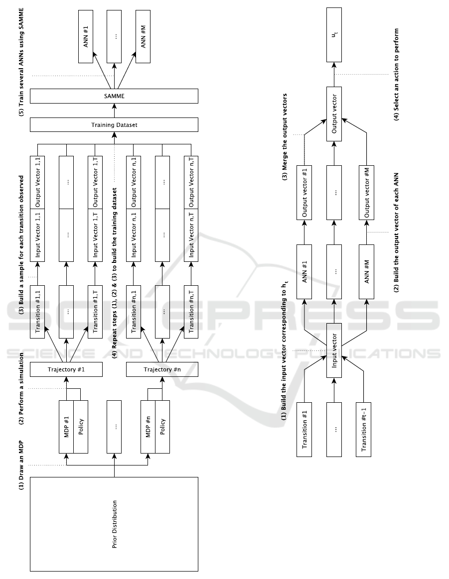
Figure 1: ANN-BRL - Offline phase.
ommended action > pair is a sample of the training
dataset.
A history is a series of transitions whose size is
Figure 2: ANN-BRL - Online phase.
unbounded, but ANNs can only be fed up with input
vectors of a fixed size. To address this issue, histo-
ries are processed into fixed-size input vectors prior
to training our model. This procedure is described in
Section 4.2.
More specifically, the ANNs are built iteratively
by using SAMME — an Adaboosting algorithm. It
consists in modifying the training dataset in order to
increase the weights of the samples misclassified by
the ANNs built previously. Section 4.3 details the
SAMME algorithm and the necessary changes to fit
the BRL setting.
Moreover, we also pseudo-code descriptions in
Approximate Bayes Optimal Policy Search using Neural Networks
145

both offline and online phases (Algorithm 1 and Algo-
rithm 2 respectively) along with UML diagrams (Fig-
ure 1 and Figure 2 respectively).
4.1 Generation of the Training Dataset
During the offline phase, we use the prior knowledge
to generate samples which will compose the training
dataset. For a given series of observations h
t
, we con-
sider the optimal action w.r.t. the MDP from which
h
t
has been generated. In other words, we give a la-
bel of 1 to actions that are optimal when the transition
function f (.) is known, and −1 to the others.
Our dataset is, thus, filled with suboptimal rec-
ommendations, from the Bayes optimal perspective.
However, our samples are generated from multiple
MDPs which are themselves sampled from the prior
distribution. As a consequence, a history h can appear
multiple times in our dataset but with different output
vectors, because it has been generated from different
MDPs for which the labels were different. The av-
erage output vector for a history h approximates the
probability of each action u to be the optimal response
to h when f
M
(.) is known, where M ∼ p
0
M
(·). To a
certain extent, it is similar to what is done by other
BRL algorithms, such as BAMCP (Guez et al., 2012)
when it explores a specific part of the belief-states
space using Tree-Search techniques.
During the data generation phase, it is necessary
to choose which parts of the state space to explore.
Generating samples by following what is believed to
be an optimal policy is likely to provide examples in
rewarding areas of the state space, but only for the
current MDP. Since it is not possible to know in ad-
vance which MDPs our agent will encounter during
the online phase, we choose to induce some random
Algorithm 2: ANN-BRL - Online phase.
Input: Prior distribution p
0
M
(.), current history
h
t
= (x
0
,u
0
,r
0
,x
1
,· ·· ,x
t−1
,u
t−1
,r
t−1
,x
t
), classifier
C (.)
Output: u
t
, the action to perform at time-step t
{Compute the input vector}
ϕ
t
← Reprocess h
t
input ← ϕ
t
{Compute the output vector}
out put ← C (input)
{Choose action u
t
w.r.t. the output vector}
k ← k maximising out put
(·)
u
t
← u
(k)
exploration in the data generation process. More pre-
cisely, we define an ε-Optimal agent, which makes
optimal decisions
2
w.r.t. to the MDP with a probabil-
ity 1−ε, and random decisions otherwise. By varying
the value of 0 < ε < 1 from one simulation to another,
we are able to cover the belief-states space more effi-
ciently than using a random agent.
4.2 Reprocess of a History
The raw input fed to our model is h
t
, an ordered se-
ries of observations up to time t. In order to simplify
the problem and reduce training time, a data prepro-
cessing step is applied to reduce h
t
to a fixed number
of features ϕ
h
t
= [ ϕ
(1)
h
t
,. .. ,ϕ
(N)
h
t
], N ∈ N. There are
two types of features that are considered in this paper:
Q-values and transition counters.
Q-values are obtained by building an approxima-
tion of the current MDP from h
t
and computing its
Q-function, thanks to the well-known Q-Iteration al-
gorithm (Sutton and Barto, 1998). Each Q-value de-
fines a different feature:
ϕ
h
t
= [ Q
h
t
(x
(1)
,u
(1)
), ... , Q
h
t
(x
(n
X
)
,u
(n
U
)
) ]
A transition counter represents the number of occur-
rences of specific transition in h
t
. Let C
h
t
(< x,u,x
0
>)
be the transition counter of transition < x,u,x
0
>. The
number of occurrences of all transitions defines the
following features:
ϕ
h
t
= [ C
h
t
(< x
(1)
,u
(1)
,x
(1)
>), ... ,
C
h
t
(< x
(n
X
)
,u
(n
U
)
,x
(n
X
)
>) ] (2)
At this stage, we computed a set of features which do
not take into account the order of appearance of each
transition. We consider that this order is not necessary
as long as the current state x
t
is known. In this paper,
two different cases have been studied:
1. Q-values: We consider the set of all Q-values de-
fined above. However, in order to take x
t
into ac-
count, those which are not related to x
t
are dis-
carded.
ϕ
h
t
= [ Q
h
t
(x
t
,u
(1)
), ... , Q
h
t
(x
t
,u
(n
U
)
) ]
2. Transition counters: We consider the set of all
transition counters defined above to which we add
x
t
as an extra feature.
ϕ
h
t
= [ C
h
t
(< x
(1)
,u
(1)
,x
(1)
>), ... ,
C
h
t
(< x
(n
X
)
,u
(n
U
)
,x
(n
X
)
>), x
t
] (3)
2
By optimal we mean the agent knows the transition matrix
of the MDP, and solve it in advance.
ICAART 2017 - 9th International Conference on Agents and Artificial Intelligence
146

4.3 Model Definition and Training
The policy is now built from the training dataset by
supervised learning on the multi-class classification
problem where the classes c are the actions, and the
vectors v are the histories. SAMME has been chosen
to address this problem. It is a boosting algorithm
which directly extends Adaboost from the two-class
classifcation problem to the multi-class case. As a
reminder, a full description of SAMME is provided
in Appendix 6.2.
SAMME builds iteratively a set of weak classifiers
in order to build a strong one. In this paper, the weak
classifiers are neural networks in the form of multi-
layer perceptrons (MLPs). SAMME algorithm aims
to allow the training of a weak classifier to focus on
the samples misclassified by the previous weak clas-
sifiers. This results in associating weights to the sam-
ples which reflect how bad the previous weak classi-
fiers are for this sample.
MLPs are trained by backpropagation
3
, which
does not support weighted samples. Schwenk et al.
presented different resampling approaches to address
this issue with neural networks in (Schwenk and Ben-
gio, 2000). The approach we have chosen sam-
ples from the dataset by interpreting the (normalised)
weights as probabilities. Algorithm 3 describes it for-
mally.
One of the specificities of the BRL formalisation
lies in the definition of the classification error δ of a
specific sample. This value is critical for SAMME in
the evaluation of the performances of an MLP and the
Algorithm 3: Resampling algorithm.
Input: The original training dataset DataSet (size
= N), a set of weights w
1
,. .. ,w
N
Output: A new training dataset DataSet
0
(size =
p)
{Normalise w
k
such that 0 ≤ ¯w
k
≤ 1 and
∑
k
¯w
k
= 1}
for i = 1 to N do
¯w
k
←
w
k
∑
k
0
w
k
0
end for
{Resample DataSet}
for i = 1 to p do
DataSet
0
(i) ← Draw a sample s from DataSet
{P(s = DataSet(k)) is equal to ¯w
k
,∀k)}
end for
3
In order to avoid overfitting, the dataset is divided into two
sets: a learning set (LS) and a validation set (VS). The
training is terminated once it begins to be less efficient on
VS. The samples are distributed 2/3 for LS and 1/3 for VS.
tuning of the sample weights. Our MLPs do not rec-
ommend specific actions, but rather give a confidence
score to each one. As a consequence, different ac-
tions can receive the same level of confidence by our
MLP(s), in which case the agent will break the tie by
selecting one of those actions randomly. Therefore,
we define the classification error δ as the probability
for an agent following a weak classifier C
0
(.) (= an
MLP) to select the class c associated to a sample v
(< v,c > being an < history, recommended action >
pair):
u
∗
= u
(c)
, ˆp = C
0
(v)
ˆ
U = {u ∈ U | u = argmax
u
ˆp
u
}
δ =
|
ˆ
U \{u
∗
}|
|
ˆ
U|
5 EXPERIMENTS
5.1 Experimental Protocol
In order to empirically evaluate our algorithm, it is
necessary to measure its expected return on a test dis-
tribution p
M
, after an offline training on a prior distri-
bution p
0
M
. Given a policy π, we denote this expected
return J
π(p
0
M
)
p
M
= E
M∼p
M
(·)
J
π(p
0
M
)
M
. In practice, we
can only approximate this value. The steps to eval-
uate an agent π are defined as follows:
1. Train π offline on p
0
M
2. Sample N MDPs from the test distribution p
M
4
3. For each sampled MDP M, compute estimate of
J
π(p
0
M
)
M
4. Use these values to compute an empirical estimate
of J
π(p
0
M
)
p
M
To estimate J
π(p
0
M
)
M
, the expected return of agent π
trained offline on p
0
M
, we sample one trajectory on the
MDP M, and compute the truncated cumulated return
up to time T. The constant T is chosen so that the
approximation error is bounded by ε = 0.01.
Finally, to estimate our comparison criterion
J
π(p
0
M
)
p
M
, we compute the empirical average of the algo-
rithm performance over N different MDPs, sampled
from p
M
. For all our experiments, we report the mea-
sured values along with the corresponding 0.95 confi-
dence interval.
4
In practice, we can only sample a finite number of trajec-
tories, and must rely on estimators to compare algorithms.
Approximate Bayes Optimal Policy Search using Neural Networks
147

The results will allow us to identify, for each ex-
periment, the most suitable algorithm(s) depending
on the constraints the agents must satisfy. Note that
this protocol has been first presented in more details
in (Castronovo et al., 2015).
5.2 Algorithms Comparison
In our experiment, the following algorithms have
been tested, from the most elementary to the state-
of-the-art BRL algorithms: Random, ε-Greedy, Soft-
max, OPPS-DS (Castronovo et al., 2012; Castronovo
et al., 2014), BAMCP (Guez et al., 2012), BFS3 (As-
muth and Littman, 2011), SBOSS (Castro and Pre-
cup, 2010), and BEB (Kolter and Ng, 2009a). For de-
tailed information on an algorithm and its parameters,
please refer to the Appendix 6.1.
Most of the above algorithms are not any-time
methods, i.e. they cannot be interrupted at an arbi-
trary time and yield a sensible result. Given an ar-
bitrary time constraint, some algorithms may just be
unable to yield anything. And out of those that do
yield a result, some might use longer time than others.
To give a fair representation of the results, we simply
report, for each algorithm and each test problem, the
recorded score (along with confidence interval), and
the computation time needed. We can then say, for
a given time constraint, what the best algorithms to
solve any problem from the benchmark are.
5.3 Benchmarks
In our setting, the transition matrix is the only ele-
ment which differs between two MDPs drawn from
the same distribution. Generating a random MDP is,
therefore, equivalent to generating a random transi-
tion matrix. In the BRL community, a common dis-
tribution used to generate such matrices is the Flat
Dirichlet Multinomial distribution (FDM). It is cho-
sen for the ease of its Bayesian updates. A FDM is
defined by a parameter vector that we call θ.
We study two different cases: when the prior
knowledge is accurate, and when it is not. In the for-
mer, the prior distribution over MDPs, called p
θ
0
M
(.),
is exactly equal to the test distribution that is used dur-
ing online training, p
θ
M
(.). In the latter, the inaccu-
racy of the prior means that p
θ
0
M
(.) 6= p
θ
M
(.).
Sections 5.3.1, 5.3.2 and 5.3.3 describes the three
distributions considered for this study.
5.3.1 Generalised Chain Distribution
The Generalised Chain (GC) distribution is inspired
from the 5-states chain problem (5 states, 3 ac-
(a) The GC distribution.
(b) The GDL distribution. (c) The Grid distribution.
Figure 3: Studied distributions for benchmarking.
tions) (Dearden et al., 1998). The agent starts at state
1, and has to go through state 2, 3 and 4 in order to
reach the last state, state 5, where the best rewards are.
This cycle is illustrated in Figure 3(a).
5.3.2 Generalised Double-Loop Distribution
The Generalised Double-Loop (GDL) distribution is
inspired from the double-loop problem (9 states, 2 ac-
tions) (Dearden et al., 1998). Two loops of 5 states
are crossing at state 1 (where the agent starts) and one
loop yields more rewards than the other. This problem
is represented in Figure 3(b).
5.3.3 Grid Distribution
The Grid distribution is inspired from the Dearden’s
maze problem (25 states, 4 actions) (Dearden et al.,
1998). The agent is placed at a corner of a 5x5 grid
(the S cell), and has to reach the goal corner (the G
cell). The agent can perform 4 different actions, cor-
responding to the 4 directions (up, down, left, right),
but the actual transition probabilities are conditioned
by the underlying transition matrix. This benchmark
is illustrated in Figure 3(c).
5.4 Results
For each experiment, we tested each algorithm with
several values for their parameter(s). The values con-
sidered in this paper are detailed in Appendix 6.1.
Three pieces of information have been measured for
each test: (i) an empirical score, obtained by testing
the agent on 500 MDPs drawn from the test distri-
bution
5
; (ii) a mean online computation time, corre-
sponding to the mean time taken by the agent for per-
forming an action; (iii) an offline computation time,
5
The same MDPs are used for comparing the agents. This
choice has been made to reduce drastically the variance of
the mean score.
ICAART 2017 - 9th International Conference on Agents and Artificial Intelligence
148

1e-06
1e-05
1e-04
1e-03
1e-02
1e-01
1e+00
1e+01
1e+02
1e+03
1e-04 1e-02 1e+00 1e+02
Offline time bound (in m)
Online time bound (in ms)
GC Experiment
Random
e-Greedy
Soft-max
OPPS-DS
BAMCP
BFS3
SBOSS
BEB
ANN-BRL (Q)
ANN-BRL (C)
1e-06
1e-04
1e-02
1e+00
1e+02
1e-06 1e-04 1e-02 1e+00
Offline time bound (in m)
Online time bound (in ms)
GDL Experiment
Random
e-Greedy
Soft-max
OPPS-DS
BAMCP
BFS3
SBOSS
BEB
ANN-BRL (Q)
ANN-BRL (C)
1e-06
1e-05
1e-04
1e-03
1e-02
1e-01
1e+00
1e+01
1e+02
1e+03
1e-08 1e-06 1e-04 1e-02
Offline time bound (in m)
Online time bound (in ms)
Grid Experiment
Random
e-Greedy
Soft-max
OPPS-DS
BAMCP
BFS3
SBOSS
BEB
ANN-BRL (Q)
ANN-BRL (C)
Figure 4: Best algorithms w.r.t offline/online periods (accurate case).
1e-06
1e-05
1e-04
1e-03
1e-02
1e-01
1e+00
1e+01
1e+02
1e+03
1e-04 1e-02 1e+00 1e+02
Offline time bound (in m)
Online time bound (in ms)
GC Experiment
Random
e-Greedy
Soft-max
OPPS-DS
BAMCP
BFS3
SBOSS
BEB
ANN-BRL (Q)
ANN-BRL (C)
1e-06
1e-05
1e-04
1e-03
1e-02
1e-01
1e+00
1e+01
1e+02
1e+03
1e-06 1e-04 1e-02 1e+00
Offline time bound (in m)
Online time bound (in ms)
GDL Experiment
Random
e-Greedy
Soft-max
OPPS-DS
BAMCP
BFS3
SBOSS
BEB
ANN-BRL (Q)
ANN-BRL (C)
1e-06
1e-04
1e-02
1e+00
1e+02
1e-08 1e-06 1e-04 1e-02
Offline time bound (in m)
Online time bound (in ms)
Grid Experiment
Random
e-Greedy
Soft-max
OPPS-DS
BAMCP
BFS3
SBOSS
BEB
ANN-BRL (Q)
ANN-BRL (C)
Figure 5: Best algorithms w.r.t offline/online time (inaccurate case).
Table 1: Best algorithms w.r.t Performance (accurate
case).
Agent Score on GC Score on GDL Score on Grid
Random 31.12 ± 0.90 2.79 ± 0.07 0.22 ± 0.06
e-Greedy 40.62 ± 1.55 3.05 ± 0.07 6.90 ± 0.31
Soft-Max 34.73 ± 1.74 2.79 ± 0.10 0.00 ± 0.00
OPPS-DS 42.47 ± 1.91 3.10 ± 0.07 7.03 ± 0.30
BAMCP 35.56 ± 1.27 3.11 ± 0.07 6.43 ± 0.30
BFS3 39.84 ± 1.74 2.90 ± 0.07 3.46 ± 0.23
SBOSS 35.90 ± 1.89 2.81 ± 0.10 4.50 ± 0.33
BEB 41.72 ± 1.63 3.09 ± 0.07 6.76 ± 0.30
ANN-BRL (Q) 42.01 ± 1.80 3.11 ± 0.08 6.15 ± 0.31
ANN-BRL (C) 35.95 ± 1.90 2.81 ± 0.09 4.09 ± 0.31
Table 2: Best algorithms w.r.t Performance (inaccurate
case).
Agent Score on GC Score on GDL Score on Grid
Random 31.67 ± 1.05 2.76 ± 0.08 0.23 ± 0.06
e-Greedy 37.69 ± 1.75 2.88 ± 0.07 0.63 ± 0.09
Soft-Max 34.75 ± 1.64 2.76 ± 0.10 0.00 ± 0.00
OPPS-DS 39.29 ± 1.71 2.99 ± 0.08 1.09 ± 0.17
BAMCP 33.87 ± 1.26 2.85 ± 0.07 0.51 ± 0.09
BFS3 36.87 ± 1.82 2.85 ± 0.07 0.42 ± 0.09
SBOSS 38.77 ± 1.89 2.86 ± 0.07 0.29 ± 0.07
BEB 38.34 ± 1.62 2.88 ± 0.07 0.29 ± 0.05
ANN-BRL (Q) 38.76 ± 1.71 2.92 ± 0.07 4.29 ± 0.22
ANN-BRL (C) 36.30 ± 1.82 2.84 ± 0.08 0.91 ± 0.15
corresponding to the time consumed by the agent
while training on the prior distribution
6
.
Each of the plots in Fig. 4 and Fig. 5 present a 2-
D graph, where the X-axis represents a mean online
computation time constraint, while the Y-axis repre-
sents an offline computation time constraint. For each
point of the graph: (i) all agents that do not satisfy
the constraints are discarded; (ii) for each algorithm,
the agent leading to the best performance in average
is selected; (iii) the list of agents whose performances
are not significantly different is built. For this pur-
6
Notice that some agents do not require an offline training
phase.
pose, a paired sampled Z-test (with a confidence level
of 95%) has been used to discard the agents which
are significantly worst than the best one. Since sev-
eral algorithms can be associated to a single point,
several boxes have been drawn to gather the points
which share the same set of algorithms.
5.4.1 Accurate Case
In Table 1, it is noted that ANN-BRL (Q)
7
gets ex-
tremely good scores on the two first benchmarks.
When taking into account time constraints, ANN-
7
Refers to ANN-BRL using Q-values as its features.
Approximate Bayes Optimal Policy Search using Neural Networks
149

BRL (Q) requires a slightly higher offline time bound
to be on par with OPPS, and can even surpass it on
the last benchmark as shown in Fig. 4.
ANN-BRL (C)
8
is significantly less efficient than
ANN-BRL (Q) on the first and last benchmarks. The
difference is less noticeable in the second one.
5.4.2 Inaccurate Case
Similar results have been observed for the inaccurate
case and can be shown in Fig. 5 and Table 2 except for
the last benchmark : ANN-BRL (Q) obtained a very
high score, 4 times larger than the one measured for
OPPS-DS. It is even more noteworthy that such a dif-
ference is observed on the most difficult benchmark.
In terms of time constraints, ANN-BRL (Q) is still
very close to OPPS-DS except for the last benchmark,
where ANN-BRL (Q) is significantly better than the
others above certain offline/online time periods.
Another difference is that even though ANN-BRL
(C) is still outperformed by ANN-BRL (Q), Fig. 5 re-
veals some cases where ANN-BRL (C) outperforms
(or is on par with) all other algorithms considered.
This occurs because ANN-BRL (C) is faster than
ANN-BRL (Q) during the online phase, which allows
it to comply with smaller online time bounds.
6 CONCLUSION AND FUTURE
WORK
We developed ANN-BRL, an offline policy-search al-
gorithm for addressing BAMDPs. As shown by our
experiments, ANN-BRL obtained state-of-the-art per-
formance on all benchmarks considered in this paper.
In particular, on the most challenging benchmark
9
, a
score 4 times higher than the one measured for the
second best algorithm has been observed. Moreover,
ANN-BRL is able to make online decisions faster
than most BRL algorithms.
Our idea is to define a parametric policy as an
ANN, and train it using backpropagation algorithm.
This requires a training set made of observations-
action pairs and in order to generate this dataset,
several simulations have been performed on MDPs
drawn from prior distribution. In theory, we should la-
bel each example with a Bayes optimal action. How-
ever, those are too expensive to compute for the whole
dataset. Instead, we chose to use optimal actions un-
der full observability hypothesis. Due to the mod-
ularity of our approach, a better labelling technique
8
Refers to ANN-BRL using transition counters as its fea-
tures.
9
Grid benchmark with a uniform prior.
could easily be integrated in ANN-BRL, and may
bring stronger empirical results.
Moreover, two types of features have been con-
sidered for representing the current history: Q-values
and transition counters. The use of Q-values allows
to reach state-of-the-art performance on most bench-
marks and outperfom all other algorithms on the most
difficult one. On the contrary, computing a good pol-
icy from transition counters only is a difficult task to
achieve, even for Artificial Neural Networks. Never-
theless, we found that the difference between this ap-
proach and state-of-the-art algorithms was much less
noticeable when prior distribution differs from test
distribution, which means that at least in some cases,
it is possible to compute efficient policies without re-
lying on online computationally expensive tools such
as Q-values.
An important future contribution would be to
provide theoretical error bounds in simple problems
classes, and to evaluate the performance of ANN-
BRL on larger domains that other BRL algorithms
might not be able to address.
ACKNOWLEDGEMENTS
Micha
¨
el Castronovo acknowledges the financial sup-
port of the FRIA.
REFERENCES
Asmuth, J., Li, L., Littman, M., Nouri, A., and Wingate,
D. (2009). A Bayesian sampling approach to explo-
ration in Reinforcement Learning. In Proceedings of
the Twenty-Fifth Conference on Uncertainty in Artifi-
cial Intelligence (UAI), pages 19–26. AUAI Press.
Asmuth, J. and Littman, M. (2011). Approaching Bayes-
optimalilty using Monte-Carlo tree search. In Pro-
ceedings of the 21st International Conference on Au-
tomated Planning and Scheduling.
Castro, P. S. and Precup, D. (2010). Smarter sam-
pling in model-based bayesian reinforcement learn-
ing. In Machine Learning and Knowledge Discovery
in Databases, pages 200–214. Springer.
Castronovo, M., Ernst, D., Couetoux, A., and Fonteneau, R.
(2015). Benchmarking for Bayesian Reinforcement
Learning. Submitted.
Castronovo, M., Fonteneau, R., and Ernst, D. (2014).
Bayes Adaptive Reinforcement Learning versus Off-
line Prior-based Policy Search: an Empirical Com-
parison. 23rd annual machine learning conference
of Belgium and the Netherlands (BENELEARN 2014),
pages 1–9.
Castronovo, M., Maes, F., Fonteneau, R., and Ernst, D.
(2012). Learning exploration/exploitation strategies
ICAART 2017 - 9th International Conference on Agents and Artificial Intelligence
150

for single trajectory Reinforcement Learning. Journal
of Machine Learning Research (JMLR), pages 1–9.
Dearden, R., Friedman, N., and Russell, S. (1998).
Bayesian Q-learning. In Proceedings of Fifteenth Na-
tional Conference on Artificial Intelligence (AAAI),
pages 761–768. AAAI Press.
Duff, M. O. (2002). Optimal Learning: Computational
procedures for Bayes-adaptive Markov decision pro-
cesses. PhD thesis, University of Massachusetts
Amherst.
Fonteneau, R., Busoniu, L., and Munos, R. (2013). Opti-
mistic planning for belief-augmented markov decision
processes. In Adaptive Dynamic Programming And
Reinforcement Learning (ADPRL), 2013 IEEE Sym-
posium on, pages 77–84. IEEE.
Guez, A., Silver, D., and Dayan, P. (2012). Efficient Bayes-
adaptive Reinforcement Learning using sample-based
search. In Neural Information Processing Systems
(NIPS).
Guez, A., Silver, D., and Dayan, P. (2013). Scalable and
efficient bayes-adaptive reinforcement learning based
on monte-carlo tree search. Journal of Artificial Intel-
ligence Research, pages 841–883.
Kaelbling, L., Littman, M., and Cassandra, A. (1998). Plan-
ning and acting in partially observable stochastic do-
mains. Artificial Intelligence, 101(12):99 – 134.
Kearns, M., Mansour, Y., and Ng, A. Y. (2002). A sparse
sampling algorithm for near-optimal planning in large
Markov decision processes. Machine Learning, 49(2-
3):193–208.
Kocsis, L. and Szepesv
´
ari, C. (2006). Bandit based Monte-
Carlo planning. European Conference on Machine
Learning (ECML), pages 282–293.
Kolter, J. Z. and Ng, A. Y. (2009a). Near-Bayesian explo-
ration in polynomial time. In Proceedings of the 26th
Annual International Conference on Machine Learn-
ing.
Kolter, J. Z. and Ng, A. Y. (2009b). Near-bayesian explo-
ration in polynomial time. In Proceedings of the 26th
Annual International Conference on Machine Learn-
ing, pages 513–520. ACM.
Martin, J. J. (1967). Bayesian decision problems and
markov chains. ”Originally submitted as a Ph.D. the-
sis [Massachusetts Institute of Technology, 1965]”.
Schwenk, H. and Bengio, Y. (2000). Boosting Neural Net-
works. Neural Comp., 12(8):1869–1887.
Silver, E. A. (1963). Markovian decision processes with
uncertain transition probabilities or rewards. Techni-
cal report, DTIC Document.
Sutton, R. S. and Barto, A. G. (1998). Reinforcement learn-
ing: An introduction, volume 1. MIT press Cam-
bridge.
Walsh, T. J., Goschin, S., and Littman, M. L. (2010). Inte-
grating sample-based planning and model-based rein-
forcement learning. In AAAI.
Wang, Y., Won, K. S., Hsu, D., and Lee, W. S. (2012).
Monte carlo bayesian reinforcement learning. arXiv
preprint arXiv:1206.6449.
Zhang, T., Kahn, G., Levine, S., and Abbeel, P. (2015).
Learning deep control policies for autonomous aerial
vehicles with mpc-guided policy search. CoRR,
abs/1509.06791.
Zhu, J., Zou, H., Rosset, S., and Hastie, T. (2009). Multi-
class adaboost. Statistics and its Interface, 2(3):349–
360.
APPENDIX
6.1 BRL Algorithms
Each algorithm considered in our experiments is de-
tailed precisely. For each algorithm, a list of “reason-
able” values is provided to test each of their parame-
ters. When an algorithm has more than one parameter,
all possible parameter combinations are tested.
6.1.1 Random
At each time-step t, the action u
t
is drawn uniformly
from U .
6.1.2 ε-Greedy
The ε-Greedy agent maintains an approximation of
the current MDP and computes, at each time-step,
its associated Q-function. The selected action is
either selected randomly (with a probability of ε
(1 ≥ ε ≥ 0), or greedily (with a probability of 1 − ε)
with respect to the approximated model.
Tested Values:
ε ∈ {0.0, 0.1,0.2,0.3,0.4, 0.5, 0.6,0.7,0.8,0.9,1.0}.
6.1.3 Soft-max
The Soft-max agent maintains an approximation of
the current MDP and computes, at each time-step, its
associated Q-function. The selected action is selected
randomly, where the probability to draw an action u is
proportional to Q(x
t
,u). The temperature parameter
τ allows to control the impact of the Q-function
on these probabilities (τ → 0
+
: greedy selection;
τ → +∞: random selection).
Tested Values:
τ ∈ {0.05,0.10,0.20, 0.33, 0.50,1.0,2.0,3.0, 5.0, 25.0}.
6.1.4 OPPS
Given a prior distribution p
0
M
(.) and an E/E strategy
space S , the Offline, Prior-based Policy Search
algorithm (OPPS) identify a strategy π
∗
∈ S which
maximises the expected discounted sum of returns
Approximate Bayes Optimal Policy Search using Neural Networks
151

over MDPs drawn from the prior. The OPPS
for Discrete Strategy spaces algorithm (OPPS-
DS) (Castronovo et al., 2012; Castronovo et al.,
2014) formalises the strategy selection problem for a
discrete strategy space of index-based strategies. The
E/E strategy spaces tested are the ones introduced
in (Castronovo et al., 2015) and are denoted by
F
2
,F
3
,F
4
,F
5
,F
6
. β is a parameter used during the
strategy selection.
Tested Values:
S ∈ {F
2
,F
3
,F
4
,F
5
,F
6
}
10
,
β ∈ {50,500, 1250,2500,5000, 10
4
,10
5
,10
6
}.
6.1.5 BAMCP
Bayes-adaptive Monte Carlo Planning
(BAMCP) (Guez et al., 2012) is an evolution of
the Upper Confidence Tree algorithm (UCT) (Kocsis
and Szepesv
´
ari, 2006), where each transition is sam-
pled according to the history of observed transitions.
The principle of this algorithm is to adapt the UCT
principle for planning in a Bayes-adaptive MDP,
also called the belief-augmented MDP, which is an
MDP obtained when considering augmented states
made of the concatenation of the actual state and the
posterior. BAMCP relies on two parameters: (i) K,
which defines the number of nodes created at each
time-step, and (ii) depth defines the depth of the tree.
Tested Values:
K ∈ {1,500, 1250,2500, 5000,10000,25000},
depth ∈ {15,25,50}.
6.1.6 BFS3
The Bayesian Forward Search Sparse Sampling
(BFS3) (Asmuth and Littman, 2011) is a BRL algo-
rithm whose principle is to apply the principle of the
FSSS (Forward Search Sparse Sampling, see (Kearns
et al., 2002)) algorithm to belief-augmented MDPs.
It first samples one model from the posterior, which
is then used to sample transitions. The algorithm then
relies on lower and upper bounds on the value of each
augmented state to prune the search space. K defines
the number of nodes to develop at each time-step, C
defines the branching factor of the tree, and finally
depth controls its maximal depth.
Tested Values:
10
The number of arms k is always equal to the number of
strategies in the given set. For your information: |F
2
| =
12,|F
3
| = 43, |F
4
| = 226, |F
5
| = 1210, |F
6
| = 7407
K ∈ {1,500, 1250,2500, 5000,10000},
C ∈ {2, 5,10, 15}, depth ∈ {15,25, 50}.
6.1.7 SBOSS
The Smarter Best of Sampled Set (SBOSS) (Castro
and Precup, 2010) is a BRL algorithm which relies
on the assumption that the model is sampled from
a Dirichlet distribution. Based on this assumption,
it derives uncertainty bounds on the value of state
action pairs. Following this step, it uses those
bounds to decide the number of models to sample
from the posterior, and the frequency with which
the posterior should be updated in order to reduce
the computational cost of Bayesian updates. The
sampling technique is then used to build a merged
MDP, as in (Asmuth et al., 2009), and to derive
the corresponding optimal action with respect to
that MDP. The number of sampled models is deter-
mined dynamically with a parameter ε, while the
re-sampling frequency depends on a parameter δ.
Tested Values:
ε ∈ {1.0, 1e − 1,1e − 2, 1e − 3,1e − 4,1e − 5, 1e − 6},
δ ∈ {9,7,5,3, 1, 1e−1,1e−2,1e−3,1e−4, 1e−5, 1e−6}.
6.1.8 BEB
The Bayesian Exploration Bonus (BEB) (Kolter and
Ng, 2009a) is a BRL algorithm that builds, at each
time-step t, the expected MDP given the current pos-
terior. Before solving this MDP, it computes a new
reward function ρ
(t)
BEB
(x,u, y) = ρ
M
(x,u, y) +
β
c
(t)
<x,u,y>
,
where c
(t)
<x,u,y>
denotes the number of times transition
< x,u, y > has been observed at time-step t. This
algorithm solves the mean MDP of the current poste-
rior, in which we replaced ρ
M
(·,·,·) by ρ
(t)
BEB
(·,·, ·),
and applies its optimal policy on the current MDP for
one step. The bonus β is a parameter controlling the
E/E balance.
Tested Values:
β ∈ {0.25,0.5, 1,1.5,2, 2.5,3, 4,8,16}.
6.1.9 ANN-BRL
The Artificial Neural Network for Bayesian Rein-
forcement Learning algorithm (ANN-BRL) is fully
described in Section 4. It samples n MDPs from
prior distribution, and generates 1 trajectory for each
MDP drawn. The transitions are then used to build
training data (one SL sample per transition), and
ICAART 2017 - 9th International Conference on Agents and Artificial Intelligence
152

several ANNs are trained on this dataset by SAMME
and backpropagation
11
. The training is parametrised
by n
h
, the number of neurons on the hidden layer
of the ANN
12
, p, the number of samples resampled
from the original training set at each epoch, ε, the
learning rate used during the training, r, the maximal
number of epoch steps during which the error on VS
can increase before stopping the backpropagation
training, and M, the maximal number of ANNs built
by SAMME. When interacting with an MDP, the
BRL agent uses the ANN trained during the offline
phase to determine which action to perform.
Fixed Parameters:
n = 750, p = 5T
13
, ε = 1e−3, r = 1000.
Tested Values:
n
h
∈ {10, 30,50}, M ∈ {1,50,100},
ϕ = {[ Q-values not related to x
t
],
[Transition counters,current state ]}.
6.2 SAMME Algorithm
A multi-class classification problem consists to find
a rule C (.) which associates a class c ∈ {1,. .., K} to
any vector v ∈ R
n
, n ∈ N. To achieve this task, we are
given a set of training samples < v
(1)
,c
(1)
>,. .. ,<
v
(N)
,c
(N)
>, from which a classification rule has to be
inferred.
SAMME is a boosting algorithm whose goal
is to build iteratively a set of weak classifiers
C
0(1)
(.),. .. ,C
0(M)
: R
n
→ R
K
, and combine them lin-
early in order to build a strong classifier C (.). In our
case, the weak classifiers are Multilayer Perceptrons
(MLPs).
C (h) =
1
M
M
∑
m=1
α
(m)
C
0(m)
(h),
where α
(1)
.. .α
(M)
are chosen to minimise the
classification error.
Given a set of training samples < v
(1)
,c
(1)
>
,. .. ,< v
(N)
,c
(N)
>, we associate a weight w
i
to each
11
2/3 for the learning set (LS) and 1/3 for the validation set
(VS).
12
In this paper, we only consider 3-layers ANNs in order to
build weak classifiers for SAMME.
13
The number of samples in LS is equal to n × T = 500T .
We resample 1% of LS at each epoch, which equals to
5T .
sample. Let err(C
0
(.)) be the weighted classification
error of a classifier C
0
(.) :
err(C
0
(.)) =
1
∑
N
i=1
w
i
N
∑
i=1
w
i
δ
C
0
i
,
where δ
C
0
i
is the classification error of C
0
(.) for
< v
(i)
,c
(i)
>.
At each iteration m, a weak classifier is trained to
minimise the weighted classification error.
C
0(m)
(.) = arg min
C
00
(.)
err(C
00
(.))err
(m)
= err(C
0
(.))
If this classifier behaves better than a random clas-
sifier (err
(m)
< (n
U
− 1)/n
U
), we compute its coef-
ficient α
(m)
, update the weights of the samples, and
build another classifier. Otherwise, we quit.
α
(m)
= log
1 − err
(m)
err
(m)
+ log (n
U
− 1)w
i
= w
i
exp(α
(m)
δ
C
0
i
)
In other words, each new classifier will focus on
training samples misclassified by the previous classi-
fiers. Algorithm 4 presents the pseudo-code descrip-
tion for SAMME.
Algorithm 4: SAMME.
Input: A training dataset DataSet
Output: A classifier C (.)
{Initialise the weight of each sample}
N ← |DataSet|
w
(1)
i
←
1
N
,∀i ∈ {1,.. ., N}
{Train weak classifiers}
m ← 1
repeat
{Train a weak classifier}
C
0(m)
← Train a classifier on DataSet w.r.t. w
(m)
{Compute its weighted error and its coefficient}
err
(m)
←
1
∑
i
w
(m)
i
∑
i
w
(m)
i
δ
C
0
i
α
(m)
← log
1−err
(m)
err
(m)
+ log (n
U
− 1)
{Adjust the weights for the next iteration}
w
(m+1)
i
← w
(m)
i
exp(α
(m)
δ
C
0
i
), ∀i
Normalise the weights w
(m+1)
m ← m + 1
until err
(m)
≥
n
U
−1
n
U
{Stop if C
0(m)
is random}
C (.) ← { < C
0(1)
, α
(1)
>, ... , < C
0(m)
, α
(m)
> }
Approximate Bayes Optimal Policy Search using Neural Networks
153
