On a Traveling Salesman based Bilevel Programming Problem

Pablo Adasme

, Rafael Andrade

, Janny Leung

and Abdel Lisser

Departamento de Ingenier´ıa El´ectrica, Universidad de Santiago de Chile, Avenida Ecuador 3519, Santiago, Chile

Departamento de Estat´ıstica e Matem´atica Aplicada, Universidade Federal do Cear´a,

Campus do Pici, BL 910, CEP 60.455-760, Fortaleza, Cear´a, Brazil

Department of Systems Engineering & Engineering Management, Chinese University of Hong Kong,

Shatin, Hong Kong, China

Laboratoire de Recherche en Informatique, Universit´e de Paris-Sud 11, Bˆat. 650 Ada Lovelace, Paris, France

Keywords:

Bilevel Programming, Traveling Salesman Problem, Mixed Integer Linear Programming Formulations,

Iterative Sub-tour Elimination Constraint Procedure.

Abstract:

In this paper, we consider a linear bilevel programming problem where both the leader and the follower

maximize their proﬁts subject to budget constraints. Additionally, we impose a Hamiltonian cycle topology

constraint in the leader problem. In particular, models of this type can be motivated by telecommunication

companies when dealing with trafﬁc network ﬂows from one server to another one within a ring topology

framework. We transform the bilevel programming problem into an equivalent single level optimization prob-

lem that we further linearize in order to derive mixed integer linear programming (MILP) formulations. This

is achieved by replacing the follower problem with the equivalent Karush Kuhn Tucker conditions and with

a linearization approach to deal with the complementarity constraints. The topology constraint is handled by

the means of two compact formulations and an exponential one from the classic traveling salesman problem.

Thus, we compute optimal solutions and upper bounds with linear programs. One of the compact models

allows to solve instances with up to 250 nodes to optimality. Finally, we propose an iterative procedure that

allows to compute optimal solutions in remarkably less computational effort when compared to the compact

models.

1 INTRODUCTION

Bilevel programming is a two level hierarchical opti-

mization framework where the upper level problem is

referred to as the leader whilst the lower level problem

is referred to as the follower problem. In a bilevel pro-

gramming problem (BPP), we aim to ﬁnd an optimal

point such that the leader and the follower maximize

(or minimize) their respectiveobjectivefunctionssub-

ject to linking constraints. Applications concerning

BPPs arise in agriculture, economic systems, ﬁnance,

engineering, banking, transportation, network design,

management and planning to name a few. For a more

general description of BPP applications and algorith-

mic approaches to solve these problems see for in-

stance (Dempe, 2003; Floudas and Pardalos, 2001;

Migdalas et al., 1997; Thirwani and Arora, 1998; Vi-

cente et al., 1994; Wang et al., 1994).

In this paper, we consider a linear bilevel pro-

gramming problem (LBPP) where both the leader and

the follower maximize their proﬁts subject to bud-

get constraints. Additionally, we impose a Hamilto-

nian cycle topology constraint in the leader problem.

In particular, models of this type can be motivated

by telecommunication companies when dealing with

trafﬁc network ﬂows from one server to another one

within a ring topology framework. As an example,

consider the problem of ﬂow trafﬁc management in

a backbone wireless token ring network where users

connect to any node and pass their messages trough

the ring in order to reach another user which is also

connected to a node in the ring (Lee et al., 2001; Song

and Yang, 1997). In these types of networks, the traf-

ﬁc ﬂows can be signiﬁcantly large which might re-

quire more than one network operator to deal with the

ﬂow problem.

We transform the LBPP into an equivalent sin-

gle level optimization problem that we further lin-

earize in order to derive mixed integer linear pro-

gramming (MILP) formulations. This is achieved

by replacing the follower problem with the equiva-

lent Karush Kuhn Tucker (KKT) conditions and with

Adasme P., Andrade R., Leung J. and Lisser A.

On a Traveling Salesman based Bilevel Programming Problem.

DOI: 10.5220/0006190503290336

In Proceedings of the 6th International Conference on Operations Research and Enterprise Systems (ICORES 2017), pages 329-336

ISBN: 978-989-758-218-9

329

the linearization approach proposed in (Audet et al.,

1997) to deal with the complementarity slackness

conditions. The topology constraint is handled by the

means of two compact polynomial formulations and

an exponential one from the classic traveling sales-

man problem (TSP) (Gavish and Graves, 1978; Letch-

ford et al., 2013; Miller et al., 1960). Thus, we

compute optimal solutions and upper bounds with the

MILP and linear programming (LP) relaxations, re-

spectively.

Our contribution in this paper is not theoretical,

but mainly focussed on computational numerical re-

sults on a novel problem in the domain of bilevel pro-

graming. As far as we know, LBPPs including Hamil-

tonian cycle topology constraints have not been con-

sidered in the literature so far. We compare numeri-

cally the exponential model with the two compact for-

mulations for randomly generated instances. For this

purpose, ﬁrst we solve the exponential model by gen-

erating all cycle elimination constraints and then, by

using an iterative algorithmic procedure which con-

sists of adding violated cycle elimination constraints

within each iteration until no cycle is found in the cur-

rent solution. Finally, we further propose a relaxed

version of the iterative algorithm and compute tight

upper bounds as well. Our main numerical result is

to show that solving the exponential model with the

iterative procedure is by far more convenient than us-

ing the compact formulations which are more theoret-

ical based approaches. In fact, we solve to optimal-

ity instances with up to 250 nodes so far, in less than

70 seconds in average compared to the higher CPU

times required by the compact formulations. It has

been proved that BPPs are strongly NP-hard even for

the simplest case in which all the involved functions

are afﬁne. See for instance (Migdalas et al., 1997;

Scholtes, 2004). The reader is referred to the books

(Dempe, 2002; Migdalas et al., 1997) for a more gen-

eral understanding on bilevel programming.

The remaining of the paper is organized as fol-

lows. In section 2, ﬁrst we present and explain the

LBPP problem. Then, we discuss three equivalent

MILP models while using the exponential and the

two compact formulations. Subsequently, in sec-

tion 3, we present the alternative iterative procedures

which allow to obtain optimal solutions and tight up-

per bounds using the exponential model. Afterwards,

in section 4 we compare all the proposed models and

the iterative procedures with the optimal solution of

the problem. Finally, in section 5 we give the main

conclusions of the paper and provide some insight for

future research.

2 LINEAR BILEVEL AND MILP

MODELS

In this section, we present and explain the LBPP. In

particular, we use an exponential number of sub-tour

elimination constraints (SECs) to characterize the

Hamiltonian cycle condition in the leader problem.

Subsequently, we use two additional compact mod-

eling approaches from the traveling salesman prob-

lem (Gavish and Graves, 1978; Letchford et al., 2013;

Miller et al., 1960) and obtain equivalent MILP mod-

els. Let G(V, E) denote a complete graph with set of

nodes V and set of directed arcs E. Our LBPP can be

formulated as follows

: max

{ f,g,x}

(

∑

ij∈E

∑

ij∈E

)

(1)

s.t.

∑

j:i j∈E

∑

j:i j∈E

≤ c, ∀i ∈ V (2)

+ g

≤ Mx

, ∀ij ∈ E (3)

∑

j:i j∈E

= 1, ∀i ∈ V (4)

∑

j: ji∈E

= 1, ∀i ∈ V (5)

∑

ij∈E(S)

≤ |S| − 1, ∀S ⊂ V (6)

∈ {0, 1}, f

≥ 0, ∀ij ∈ E (7)

g ∈ argmax

{g}

(

∑

ij∈E

∑

ij∈E

)

(8)

∑

j:i j∈E

∑

j:i j∈E

≤ r,

∀i ∈ V (9)

≥ 0, ∀ij ∈ E (10)

In BP

, the input symmetric matrices

{C, D, A, B, H, P, Q, R} ∈ M

|V|×|V|

) and the

scalars {c, r} ∈ R

, respectively. Constraints (1)-(7)

correspond to the leader problem whereas constraints

(8)-(10) represent the follower problem. Without loss

of generality, we assume that the set V represents

servers to visit whereas the set E represents trafﬁc

links by which the network ﬂow service should be

carried out from one server to another. Thus, the bi-

nary decision variable x

= 1 if and only if the leader

company decides to use the link (i, j) and x

= 0

otherwise, ∀ij ∈ E. Similarly, the decision variables

, g

≥ 0 represent the amount of network ﬂow to

transport from i to j for the leader and follower prob-

lems, respectively. The objective functions maximize

the proﬁts for both the leader and the follower and

are given in (1) and (8), respectively. Whereas the

constraints (2) and (9) represent the costs structure

ICORES 2017 - 6th International Conference on Operations Research and Enterprise Systems

330

associated to each one of them. Constraints (7) and

(10) are domain constraints for the decision variables.

The constraints (3)-(6) characterize the Hamiltonian

cycle condition imposed in the leader problem. In

particular, the constraint (3) implies that whenever

the variable x

= 0, then the variables f

and g

must

be equal to zero ∀ij ∈ E. For this purpose, we use a

large positive BigM value denoted by M. Constraints

(4)-(5) enforce the condition that each node should

be connected to two nodes in the circuit. Finally,

constraint (6) represents SECs ∀S ⊂ V. Notice that

we do not include SECs for S ≡ V in order to allow

obtaining feasible solutions, i.e., Hamiltonian cycles.

An equivalent MILP model can be straightfor-

wardly obtained by replacing the follower problem

with the equivalent KKT conditions and by using

the linearization approach proposed in (Audet et al.,

1997) to deal with the complementarity slackness

conditions (Audet et al., 1997; Dempe, 2003). This

leads to the following equivalent MILP model

MIP

: max

{ f,g,x,λ,µ,θ,ν}

(

∑

ij∈E

∑

ij∈E

)

s.t.

∑

j:i j∈E

∑

j:i j∈E

≤ c, ∀i ∈ V

+ g

≤ Mx

, ∀ij ∈ E

∑

j:i j∈E

= 1, ∀i ∈ V

∑

j: ji∈E

= 1, ∀i ∈ V

∑

ij∈E(S)

≤ |S| − 1, ∀S ⊂ V (11)

∈ {0, 1}, f

≥ 0, ∀ij ∈ E

− λ

+ µ

= 0, ∀ij ∈ E (12)

∑

j:i j∈E

∑

j:i j∈E

≤ r, ∀i ∈ V (13)

r−

∑

j:i j∈E

−

∑

j:i j∈E

+ ν

L ≤ L,

∀i ∈ V (14)

≤ ν

L, ∀i ∈ V (15)

+ θ

L ≤ L, ∀ij ∈ E (16)

≤ θ

L, ∀ij ∈ E (17)

, µ

≥ 0∀ij ∈ E, λ

≥ 0∀i ∈ V (18)

∈ {0, 1}∀i ∈ V, θ

∈ {0, 1}∀ij ∈ E (19)

where the constraints (12) are due to the derivatives

obtained with the Lagrangian function of the follower

problem and with respect to the variables g

, ∀ij ∈ E.

The non-negative variables λ

, ∀i ∈ V and µ

, ∀ij ∈ E

are dual variables for the constraints (9) and (10), re-

spectively. The constraints (13)-(15) enforce the con-

dition that either



r−

∑

j:i j∈E

−

∑

j:i j∈E



or λ

should be equal to zero ∀i ∈ V. This is handled

with the binary variable ν

∀i ∈ V and with the large

positive value L. Similarly, the constraints (16)-(17)

enforce the condition that either µ

or g

should be

equal to zero for all ij ∈ E. This is handled with the

variables θ

∈ {0, 1}∀ij ∈ E. Finally, (18)-(19) are

domain constraints for the decision variables.

As it can be observed, the number of SECs in

MIP

is exponential. To overcome this difﬁculty, we

further consider the following MILP model which

uses a well known characterization of the feasible

space of the traveling salesman problem (Letchford

et al., 2013; Miller et al., 1960)

MIP

: max

{ f,g,x,u,λ,µ,θ,ν}

(

∑

ij∈E

∑

ij∈E

)

s.t.

∑

j:i j∈E

∑

j:i j∈E

≤ c, ∀i ∈ V

+ g

≤ Mx

, ∀ij ∈ E

∑

j:i j∈E

= 1, ∀i ∈ V

∑

j: ji∈E

= 1, ∀i ∈ V

= 1 (20)

2 ≤ u

≤ |V|, ∀i ∈ V, (i 6= 1) (21)

− u

+ 1 ≤ (|V| − 1)(1 − x

∀ij ∈ E, (i 6= 1), ( j 6= 1) (22)

∈ Z

, ∀ j ∈ V (23)

∈ {0, 1}, f

≥ 0, ∀ij ∈ E

− λ

+ µ

= 0, ∀ij ∈ E

∑

j:i j∈E

∑

j:i j∈E

≤ r, ∀i ∈ V

r−

∑

j:i j∈E

−

∑

j:i j∈E

+ ν

L ≤ L, ∀i ∈ V

≤ ν

L, ∀i ∈ V

+ θ

L ≤ L, ∀ij ∈ E

≤ θ

L, ∀ij ∈ E

, µ

≥ 0∀ij ∈ E, λ

≥ 0∀i ∈ V

∈ {0, 1}∀i ∈ V, θ

∈ {0, 1}∀ij ∈ E

where the constraints (22) ensure that, if the sales-

man travels from i to j, then the nodes i and j are ar-

ranged sequentially. These constraints together with

(20)-(21) and (23) ensure that each node is in a unique

position. A third formulation can be obtained by us-

ing the classic single commodity ﬂow formulation for

the TSP (Gavish and Graves, 1978; Letchford et al.,

2013). For this purpose, we assume that the salesman

carries |V| − 1 units of a commodity when he leaves

node 1, and delivers 1 unit of this commodity to each

node. We can deﬁne additional continuous variables

On a Traveling Salesman based Bilevel Programming Problem

331

i, j

≥ 0, ∀ij ∈ E representing the amount of the com-

modity (if any) routed directly from node i to node j.

The new MILP formulation is

MIP

: max

{ f,g,x,w,λ,µ,θ,ν}

(

∑

ij∈E

∑

ij∈E

)

s.t.

∑

j:i j∈E

∑

j:i j∈E

≤ c, ∀i ∈ V

+ g

≤ Mx

, ∀ij ∈ E

∑

j:i j∈E

= 1, ∀i ∈ V

∑

j: ji∈E

= 1, ∀i ∈ V

∑

j: ji∈E

−

∑

j>1:ij∈ E

= 1,

∀i ∈ {2, . . . , |V|} (24)

0 ≤ w

≤ (|V| − 1)x

, ∀ij ∈ E (25)

, f

≥ 0∀ij ∈ E

− λ

+ µ

= 0, ∀ij ∈ E

∑

j:i j∈E

∑

j:i j∈E

≤ r, ∀i ∈ V

r−

∑

j:i j∈E

−

∑

j:i j∈E

+ ν

L ≤ L, ∀i ∈ V

≤ ν

L, ∀i ∈ V

+ θ

L ≤ L, ∀ij ∈ E

≤ θ

L, ∀ij ∈ E

, µ

≥ 0∀ij ∈ E, λ

≥ 0∀i ∈ V

∈ {0, 1}∀i ∈ V, θ

∈ {0, 1}∀ij ∈ E

The constraints (24) ensure that one unit of the com-

modity is delivered to each node while the bounds in

(25) ensure that the commodity can ﬂow only along

arcs in the solution. Hereafter, we denote by LP

, LP

and LP

the LP relaxations of MIP

, MIP

and MIP

respectively.

In the next section, we present an alternative iter-

ative algorithmic procedure that allows to obtain op-

timal solutions and tight upper bounds for MIP

3 ITERATIVE PROCEDURE FOR

GENERATING SECS

The procedure to generate SECs can be easily adapted

using Algorithms 4.1 and 4.2 from (Adasme et al.,

2015) to MIP

. The main idea can be described as

follows. If we removeconstraints (11) from MIP

and

solve the resulting integer linear programming prob-

lem, then the underlying optimal solution induces a

graph

G that may contain a cycle with at least two

nodes. In this case, it can be detected by a depth-ﬁrst

search procedure (Cormen et al., 2009). In this pa-

per, we adapt the procedure 4.1 from (Adasme et al.,

2015) to ﬁnd cycles in directed graphs with at least 2

and up to |V|−1 nodes. In particular,if the cardinality

of a subset of nodes found with Algorithm 4.1 induc-

ing a cycle equals |V|, we do not generate the SEC,

otherwise Hamiltonian cycles would be infeasible for

the problem.

Algorithm 3.1: Iterative procedure to compute upper

bounds for MIP

Data: A problem instance of MIP

Result: An upper bound with solution

( f, g, x

, λ, µ, θ, ν) for MIP

with objective

function value z

Step 0

: Set k = 1;

Let MIP

be the problem obtained from MIP

removing the constraints (11) at iteration k;

Solve the MILP relaxation of problem MIP

and let

( f

, g

, x

, λ

, µ

, θ

, ν

) be its optimal solution of

value z

at iteration k;

Let z

= inf;

Step 1: while |z

k−1

− z

| > ε do

Construct the graph

G = (V,

E) with the rounded

solution (

, ˜g

, ˜x

, ˜µ

) obtained

from ( f

, g

, x

, λ

, µ

, θ

, ν

);

C = searchCycles(

G,V);

foreach cycle ∈ C do

Add the corresponding constraint (11) to

MIP

;

Set k = k+ 1;

Solve the MILP relaxation of problem MIP

and let ( f

, g

, x

, λ

, µ

, θ

, ν

) be its optimal

solution of value z

at iteration k;

return the solution ( f

, g

, x

, λ

, µ

, θ

, ν

, z

);

Algorithm 4.1 is used iteratively by Algorithm

4.2 in (Adasme et al., 2015) that we adapt to solve

MIP

. The procedures in Algorithms 4.1 and 4.2 can

be straightforwardly explained in more detail as fol-

lows. First, we remove constraints (11) from MIP

and solve the resulting integer optimization problem.

Consider the underlying optimal solution graph

G =

(V,

E) where V is the set of nodes and

E is the set

of arcs such that

E ⊆ E. If

G contains a cycle with

two or up to |V| − 1 nodes, then Algorithm 4.1 de-

tects it. A subset of nodes inducing a cycle deﬁnes a

new constraint (11) which cuts off this cycle from the

solution space. Problem MIP

is re-optimized taking

into account the new added constraints. This itera-

tive process goes on until the underlying current op-

timal solution of MIP

has no more cycles. Since the

number of cycles is ﬁnite, so is the number of con-

straints (11) that can be added to MIP

. Notice that

the number of SECs of type (11) that can be added to

ICORES 2017 - 6th International Conference on Operations Research and Enterprise Systems

332

MIP

is at most O(2

|V|

). Consequently, Algorithm 4.2

adapted to solve MIP

, converges to the optimal solu-

tion of the problem in at most O(2

|V|

) outer iterations.

The proof can be directly deduced from Theorem 2 in

(Adasme et al., 2015).

The aforementioned procedure can also be used

to compute upper bounds for MIP

. This proce-

dure is depicted in Algorithm 3.1 and is described

as follows. First, we remove constraints (11) from

MIP

and solve the resulting mixed integer linear

programming relaxation of MIP

obtained while re-

laxing the variables 0 ≤ x

≤ 1 ∀ij ∈ E at step 0.

Next, we search cycles in the current rounded solu-

tion 0 ≤ x

≤ 1 ∀ij ∈ E. If

G contains a cycle with

two or more nodes, then Algorithm 4.1 referred to

as “searchCycles(

G,V)” in (Adasme et al., 2015) de-

tects it. A subset of nodes inducing a cycle deﬁnes

a new constraint (11). The mixed integer program-

ming relaxation of MIP

is re-optimized taking into

account the new added constraints. This iterative pro-

cess goes on until the difference between the current

optimal objective function value z

and the previous

one z

k−1

is less than a small positive value ε.

4 PRELIMINARY NUMERICAL

RESULTS

In this section, we present preliminary numerical re-

sults. A Matlab (R2012a) program is developed using

CPLEX 12.6 to solve MIP

, MIP

and their

corresponding LP relaxations. The numerical exper-

iments have been carried out on an Intel(R) 64 bits

core (TM) with 2.6 GHz and 8 Gigabytes of RAM.

CPLEX solver is used with default options. Each en-

try in matrices {C, D, H} and in matrices {A, B, R, Q}

is randomly and uniformly distributed in the inter-

vals [0;10] and [0;5], respectively. The scalar values

c = r = 100. The BigM values M and L are set to

M = 100 and L = 10

, respectively. We set the pa-

rameter ε = 10

−8

in Algorithm 3.1. In Table 1, ﬁrst

we solve MIP

with up to 15 nodes while generat-

ing all cycle elimination constraints. Subsequently, in

Table 3, we solve MIP

with the iterative procedures

presented in section 3. We limit CPLEX to 2 hours

of CPU time in order to solve the linear models. The

legend in Table 1 is as follows. Column 1 shows the

instance number. Column 2 presents the number of

nodes. Columns 3-7 and 8-12 present the optimal so-

lution of MIP

and MIP

, the number of branch and

bound nodes used by CPLEX, the CPU time in sec-

onds to solve the MILPs and their corresponding LP

relaxations together with their CPU time in seconds,

respectively. Finally, in columns 13-14, we present

gaps we compute as

LP−Opt

Opt

∗ 100 for MIP

and

MIP

, respectively. The legend in Table 2 for MIP

is analogous to Table 1. We mention that each row in

Tables 1, 2 and 3 corresponds to the same instance.

From Tables 1, 2 and 3, we observe that the op-

timal objective function values for MIP

, MIP

and

MIP

are exactly the same. In particular, in Tables

1 and 2, we see that the CPU times are in average

signiﬁcantly lower for MIP

than for MIP

. In par-

ticular, when the instance dimensions increase. Re-

garding the number of branch and bound nodes, we

observe that CPLEX requires signiﬁcantly less nodes

for solving MIP

than for MIP

. For MIP

, the num-

ber of nodes equals zero for the instances 1-7. Notice

that CPLEX cannot ﬁnd a feasible solution within 2

hours for the instance #18 using MIP

. This is some-

how reﬂected by the number of branch and bound

nodes which is signiﬁcantly higher for MIP

than for

MIP

. Concerning the LP bounds, the LP relaxations

are slightly tighter for MIP

than for MIP

and MIP

Whereas the bounds for LP

and LP

remain nearly

the same. On the opposite, the CPU times for LP

are in average larger than for LP

, in particular for

the large size instances. We also see that CPLEX

can solve all the instances to optimality using MIP

that shows a signiﬁcantly better performance than the

rest of the MILP formulations. Finally, we mention

that we cannot solve, with the exponential model, in-

stances with more than 15 nodes due to the large num-

ber of sub-tour elimination constraints involved.

In Table 3, the legend is as follows. In column

1, we show the instance number. In columns 2-5, we

show the optimal solution obtained with the adapted

version of Algorithm 4.2 (Adasme et al., 2015), its

CPU time in seconds, the number of cycles found

with this algorithm and the number of iterations, re-

spectively. In columns 6-10, we present the upper

bounds obtained with Algorithm 3.1, its CPU time

in seconds, the number of cycles found with it, the

number of iterations, and the optimal solution found

with MIP

while using all the cycle elimination con-

straints found with Algorithm 3.1, respectively. For

the latter, we do not report the CPU time required by

CPLEX. However, we mention that for the largest size

instances (e.g. 21-22), these CPU times took less than

20 seconds. The rest of the instances were solved in

less than 2 seconds. Finally, in columns 11-12, we

provide gaps that we compute by

Opt

−Opt

Opt

∗ 100

and

Opt

−Opt

Opt

∗ 100, respectively.

From Table 3, we observe that Algorithm 4.2 can

ﬁnd the optimal solutions for all the instances. In par-

ticular, we observe that the large size instances #15-22

are solved in signiﬁcantly less CPU time compared to

On a Traveling Salesman based Bilevel Programming Problem

333

Table 1: Numerical results obtained with MIP

and MIP

# |V|

MIP

Gaps

Opt B&Bn Time (s) LP Time (s) Opt B&Bn Time (s) LP Time (s) Gap

% Gap

1 4 945.90 0 0.35 1547.52 0.35 945.90 0 0.36 1547.52 0.41 63.60 63.60

2 6 1223.95 0 0.41 1969.08 0.39 1223.95 0 0.41 1969.08 0.42 60.88 60.88

8 1574.80 0 0.37 2990.03 0.42 1574.80 0 0.37 2996.69 0.38 89.87 90.29

4 10 1992.63 0 0.53 5252.53 0.53 1992.63 29 0.34 5368.06 0.40 163.60 169.40

12 2781.27 0 1.83 5472.70 1.28 2781.27 6 0.40 5745.17 0.39 96.77 106.57

6 14 3795.17 0 7.13 6476.50 5.45 3795.17 120 0.42 6505.47 0.39 70.65 71.41

15 4233.11 0 14.74 6596.09 11.05 4233.11 0 0.39 6723.12 0.34 55.82 58.82

8 20 - - - - - 5920.61 1886 1.39 10090.09 0.39 - 70.42

9 25 - - - - - 7979.07 30 0.53 13672.93 0.38 - 71.36

30 - - - - - 11272.16 8 0.50 16961.67 0.41 - 50.47

11 40 - - - - - 14325.01 0 0.62 25545.21 0.52 - 78.33

50 - - - - - 17772.48 0 0.80 30645.26 0.55 - 72.43

13 60 - - - - - 23021.58 528 2.63 39462.28 0.86 - 71.41

70 - - - - - 28178.71 54 2.17 47919.83 1.19 - 70.06

15 80 - - - - - 32776.32 335 3.87 55799.72 1.55 - 70.24

90 - - - - - 35705.34 918 26.15 62552.35 1.90 - 75.19

17 100 - - - - - 42688.50 44278 452.83 73934.28 2.39 - 73.19

120 - - - - - * 379412 7200 86563.41 5.50 - *

19 150 - - - - - - - - 113013.27 21.22 - -

180 - - - - - - - - 139047.61 59.52 - -

21 200 - - - - - - - - 156705.84 73.85 - -

250 - - - - - - - - 201738.80 268.30 - -

-: Instance not solved.

*: No solution found with CPLEX in 2 hours.

Table 2: Numerical results obtained with MIP

MIP

Gaps

Opt B&Bn Time (s) LP Time (s) Gap

1 945.90 0 0.40 1547.52 0.37 63.60

1223.95 0 0.40 1969.08 0.37 60.88

3 1574.80 0 0.37 2996.69 0.39 90.29

1992.63 0 0.42 5361.12 0.37 169.05

5 2781.27 9 0.49 5745.17 0.39 106.57

3795.17 8 0.49 6485.70 0.42 70.89

7 4233.11 0 0.40 6723.12 0.36 58.82

5920.61 10 0.94 10047.35 0.43 69.70

9 7979.07 0 0.54 13618.52 0.41 70.68

11272.16 0 0.75 16961.67 0.45 50.47

11 14325.01 0 0.79 25538.77 0.68 78.28

17772.48 0 1.17 30645.26 0.64 72.43

13 23021.58 675 10.46 39453.01 1.05 71.37

28178.72 8 5.11 47881.09 1.83 69.92

15 32776.31 248 17.79 55799.72 2.93 70.24

16 35705.36 17 15.86 62552.35 2.53 75.19

42688.51 621 46.65 73934.28 3.75 73.19

18 50786.93 526 133.94 86493.02 17.00 70.31

66770.38 163 123.39 113003.02 58.75 69.24

20 86307.85 4168 2459.89 139046.61 211.01 61.11

93444.25 5678 6878.94 156675.69 230.30 67.67

22 122719.37 549 2017.85 201734.01 901.54 64.39

MIP

. Moreover, the number of cycles and iterations

are less or equal than 140 and 11, respectively for all

the instances. Notice that the total number of cycles

for most of the instances is huge. However, the num-

ber of cycles required by Algorithm 4.2 to ﬁnd the

optimal solution is signiﬁcantly small. In general, we

see that Algorithm 3.1 can ﬁnd tighter bounds when

compared to the models LP

and LP

. Regarding the

number of cycles required by Algorithm 3.1, we ob-

serve that this number is signiﬁcantly higher com-

pared to Algorithm 4.2. On the opposite, we see that

Algorithm 3.1 requires in average less iterations. Fi-

ICORES 2017 - 6th International Conference on Operations Research and Enterprise Systems

334

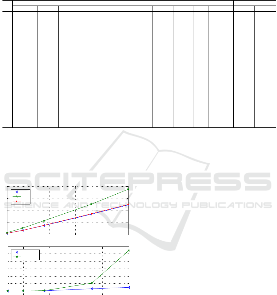
Table 3: Numerical results obtained with the iterative algorithmic procedures.

Algorithms 4.1 and 4.2 adapted from (Adasme et al., 2015) Algorithm 3.1 Gaps

Opt

Time (s) #Cycles #Iter Opt

Gap

% Gap

1 945.90 0.51 0 1 1443.61 1.09 10 2 945.90 52.62 0

2 1223.95 0.80 3 2 1899.73 0.80 8 1 1239.34 55.21 1.26

1574.80 0.76 4 2 2896.01 0.76 12 1 1574.80 83.90 0

4 1992.63 0.80 5 2 4269.07 1.08 32 2 2036.42 114.24 2.20

2781.27 1.26 8 3 4447.16 1.20 41 2 2787.50 59.90 0.22

6 3795.17 1.66 9 4 5800.14 1.26 41 2 3995.48 52.83 5.28

4233.11 1.25 8 3 5963.58 1.22 45 2 4328.84 40.88 2.26

8 5920.61 2.40 18 6 8952.44 1.23 58 2 6233.36 51.21 5.28

9 7979.07 0.89 12 2 13244.42 1.36 75 2 8441.78 65.99 5.80

11272.16 1.34 14 3 15160.96 1.51 97 2 11342.97 34.50 0.63

11 14325.01 1.63 18 3 23008.49 3.05 207 3 14661.88 60.62 2.35

17772.48 2.89 27 4 27771.65 2.95 168 2 18442.49 56.26 3.77

13 23021.58 12.30 45 11 36082.31 6.66 312 3 23959.25 56.73 4.07

28178.71 7.87 42 6 44084.55 6.28 235 2 29376.14 56.45 4.25

15 32776.31 16.27 55 9 51378.66 20.60 536 4 33437.84 56.76 2.02

35705.34 5.95 50 3 56294.82 10.57 323 2 36700.49 57.66 2.79

17 42688.50 27.17 71 10 65957.50 24.66 537 3 44117.89 54.51 3.35

50786.93 38.96 83 9 77440.29 25.01 413 2 52118.73 52.48 2.62

19 66770.38 71.56 92 9 101128.60 199.45 1090 4 68005.67 51.46 1.85

86307.85 153.10 125 11 127706.66 410.10 1007 3 87895.55 47.97 1.84

21 93444.25 122.41 127 7 141811.63 325.40 706 2 96921.84 51.76 3.72

122719.37 122.20 140 4 186448.77 948.96 919 2 126746.65 51.93 3.28

nally, we observe that solving MIP

with all the cy-

cle elimination constraints found with Algorithm 3.1

allows to compute tight bounds when compared to

the optimal solution of the problem. More precisely,

these bounds are computed with gaps which are lower

than 6% for most of the instances.

50 100 150 200 250

0.5

1.5

x 10

Number of nodes |V |.

50 100 150 200 250

200

400

600

800

1000

1200

Number of nodes |V |.

Opt

CPU (Opt

)

CPU (Opt

)

Figure 1: Average optimal solutions, upper bounds and

CPU times obtained with the iterative Algorithms 4.2 and

3.1.

In order to give more insight with respect to the

performance of Algorithms 4.2 and 3.1 when solving

MIP

. In Figure 1, we present some average numer-

ical results for 20 instances randomly generated with

dimensions of |V| = {20, 50, 90, 180, 250} nodes, re-

spectively. From Figure 1, we mainly conﬁrm the

trends observed in Table 3. We observe that in av-

erage obtaining optimal solutions with the iterative

Algorithm 4.2 is more effective than computing up-

per bounds with Algorithm 3.1 in terms of CPU time.

This is an interesting result as it conﬁrms that Algo-

rithm 4.2 allows to obtain optimal solutions for the

large scale instances more easily. More precisely, in

less CPU time than the instances presented in Table

3. Finally, we observe that the upper bounds obtained

with Algorithm 3.1 are very tight when solving MIP

with all SECs, although they are obtained at a higher

CPU time. In Figure 1, we do not plot averages for the

number of cycles and iterations as they remain nearly

the same as in Table 3 for all the instances. Similarly,

we do not plot the average CPU times for Opt

since

they are slightly larger than those obtained for Opt

5 CONCLUSIONS

In this paper, we consider a linear bilevel program-

ming problem where both the leader and the follower

maximize their proﬁts subject to budget constraints.

Additionally, we impose a Hamiltonian cycle topol-

ogy constraint in the leader problem. In particular,

models of this type can be motivated by telecom-

munication companies when dealing with trafﬁc net-

work ﬂows from one server to another one within a

ring topology framework. We transform the bilevel

programming problem into an equivalent single level

optimization problem and derive mixed integer lin-

ear programming (MILP) formulations. The topology

constraint is handled by the means of two compact

On a Traveling Salesman based Bilevel Programming Problem

335

formulations and an exponential one from the clas-

sic traveling salesman problem. Our preliminary nu-

merical results show that one of the compact models

allows to solve instances with up to 250 nodes to op-

timality with CPLEX in less than two hours. Finally,

we propose iterative proceduresthat allow to compute

optimal solutions in signiﬁcantly less computational

effort when compared to the compact models. Our

main contribution in this paper is not theoretical, but

mainly focussed on computational numerical results

on a novel problem in the domain of bilevel program-

ing. Our numerical results clearly show that solving

the exponential model with the iterative procedure is

by far more convenientthan using the compact formu-

lations which are more theoretical based approaches.

In fact, we solve to optimality instances with up to

250 nodes so far, in less than 70 seconds in average

compared to the higher CPU times required by the

compact formulations.

As part of future research, we plan to develop fur-

ther tests in order to conﬁrm the behaviour of the

proposed models and algorithms. Finally, we will

propose new stochastic models and algorithmic ap-

proaches for this type of bilevel programming prob-

lems.

ACKNOWLEDGEMENTS

The ﬁrst author acknowledges the ﬁnancial support of

the USACH/DICYT Project 061513VC DAS.

REFERENCES

Adasme, P., Andrade, R., Letournel, M., and Lisser, A.

(2015). Stochastic maximum weight forest problem.

Networks, 65:289–305.

Audet, C., Hansen, P., Jaumard, B., and Savard, G. (1997).

Links between linear bilevel and mixed 0-1 program-

ming problems. Journal of Optimization Theory and

Applications, 93:273–300.

Cormen, T. H., Leiserson, C. E., Rivest, R. L., and Stein,

C. (2009). Introduction to algorithms. MIT Press and

McGraw-Hill, Cumberland, RI, USA.

Dempe, S. (2002). Foundations of bilevel programming.

(1st ed.). Freiberg: Kluwer Academic Publishers.

Dempe, S. (2003). Annotated bibliography on bilevel pro-

gramming and mathematical programs with equilib-

rium constraints. Optimization, 52:333–359.

Floudas, C. and Pardalos, P. (2001). Encyclopedia of opti-

mization. Dordrecht: Kluwer Academic Publishers.

Gavish, B. and Graves, S. C. (1978). The travelling sales-

man problem and related problems. Operations Re-

search Centre, Massachusetts Institute of Technology.

Lee, D., Attias, R., Puri, A., Sengupta, R., Tripakis, S., and

Varaiya, P. (2001). A wireless token ring protocol

for intelligent transportation systems. In IEEE Pro-

ceedings of: Intelligent Transportation Systems, pages

1152–1157.

Letchford, A. N., Nasiri, S. D., and Theis, D. O. (2013).

Compact formulations of the steiner traveling sales-

man problem and related problems. European Journal

of Operational Research, 228:83–92.

Migdalas, A., Pardalos, P., and Varbrand, P. (1997). Multi-

level optimization: Algorithms and Applications. The

Netherlands: Kluwer Academic Publishers.

Miller, C. E., Tucker, A. W., and Zemlin, R. A. (1960). In-

teger programming formulation of traveling salesman

problems. J. Assoc. Comput. Mach., 7:326–329.

Scholtes, S. (2004). Nonconvex structures in nonlinear pro-

gramming. Operations Research, 52:368–383.

Song, J. and Yang, O. (1997). Backbone networks using

rotation counters. IEEE Transactions on Parallel and

Distributed Systems, 8:1288–1298.

Thirwani, D. and Arora, S. (1998). An algorithm for

quadratic bilevel programming problem. Interna-

tional Journal of Management and System, 14:89–98.

Vicente, L., Savard, G., and Judice, J. (1994). Descent

approaches for quadratic bilevel programming. Jour-

nal of Optimization Theory and Applications, 81:379–

399.

Wang, S., Wang, Q., and Rodriguez, R. (1994). Optimal-

ity conditions and an algorithm for linear-quadratic

bilevel programs. Optimization, 31:127–139.

ICORES 2017 - 6th International Conference on Operations Research and Enterprise Systems

336