
Concatenated Decision Paths Classification for Datasets with Small
Number of Class Labels
Ivan Mitzev and Nicolas H. Younan
Mississipi State University, Department of Electrical and Computer Engineering, Mississippi State, MS 39762, U.S.A.
ism6@msstate.edu, younan@ece.msstate.edu
Keywords: Time Series Classification, Time Series Shapelets, Combined Classifiers, Concatenated Decision Paths.
Abstract: In recent years, the amount of collected information has rapidly increased, that has led to an increasing
interest to time series data mining and in particular to the classification of these data. Traditional methods
for classification are based mostly on distance measures between the time series and 1-NN classification.
Recent development of classification methods based on time series shapelets- propose using small sub-
sections of the entire time series, which appears to be most representative for certain classes. In addition, the
shapelets-based classification method produces higher accuracies on some datasets because the global
features are more sensitive to noise than the local ones. Despite its advantages the shapelets methods has an
apparent disadvantage- slow training time. Varieties of algorithms were proposed to tackle this problem,
one of which is the concatenated decision paths (CDP) algorithm. This algorithm as initially proposed
works only with datasets with a number of class indexes higher than five. In this paper, we investigate the
possibility to use CDP for datasets with less than five classes. We also introduce improvements that shorten
the overall training time of the CDP method.
1 INTRODUCTION
Time series is very common format for presenting
collected data such as stock analysis and forecasting,
temperature changes, earthquake records among
others. In the last decade, the interest in time series
data mining increases as the amount of collected
data increases dramatically. As a result, the
technologies for indexing, classification and
clustering of time series have achieved new levels.
Traditional approaches for time series classification
require precise definition of the distance between
two time series. The variety of distance measures,
such as Euclidian distance (ED); Dynamic time
warping (DTW); Edit distance with real penalty
(ERP), among others are used along with a 1-NN
classifier to perform time series classification. Other
popular methods for time series classification
include decision trees, Bayesian networks, and
support vector machines. Recently (Ye and Keogh,
2009) introduced a new approach, called time series
shapelets. Instead of using global features to
represent the time series, this approach extracts sub-
series from the train time series which maximally
represents a certain class. As the sub-series depict a
local feature, it appears that the method produces
higher accuracies, based on the fact that the local
features are less sensitive to noise than the global
features. Despite its advantage, their method has a
very slow training time. A variety of methods had
been introduced to speed up the training process.
Some of them are discussed in Chapter 2 with more
details. One recently proposed method, named
Concatenated Decision Paths (CDP), trains decision
trees and collect their decision paths, forming a so
called decision pattern. It appears that every class
has its representative decision pattern, used for
further classification of the incoming time series. As
introduced, the method is applicable only for
datasets with more than 5 class indexes. In case of
only 2 class indexes for example, the decision
pattern will have a length equal to 1. Generally,
shorter decision patterns produce lower accuracies,
thus, the method initially is considered as not
applicable for datasets with small number of class
labels. Our recent research showed that re-training
the decision trees with the same class indexes
significantly increases the accuracy. Although- the
trees have the same class indexes, every node
appears to have its unique shapelet and split
distance, guaranteed by the randomness of the
decision tree training process. Thus, every decision
tree gives its unique decision into the final decision
pattern.
410
Mitzev, I. and Younan, N.
Concatenated Decision Paths Classification for Datasets with Small Number of Class Labels.
DOI: 10.5220/0006190004100417
In Proceedings of the 6th International Conference on Pattern Recognition Applications and Methods (ICPRAM 2017), pages 410-417
ISBN: 978-989-758-222-6
Copyright
c
2017 by SCITEPRESS – Science and Technology Publications, Lda. All rights reserved

The rest of this paper is organized as follows:
Chapter 2 reviews the most recent methods in time
series shapelets classification. Chapter 3 introduces
the CDP method and the proposed extension for
datasets with less class labels. Chapter 4 presents the
results of this research and Chapter 5 summarizes
the achievements of this work and proposes further
developments.
2 RELATED WORK
The initial implementation of the time series
shapelets classification method (Ye and Keogh,
2009) was based on the Brute Force Algorithm. The
method extracts all possible sub-sequences from all
the time series in the train dataset D and assesses
their potential to separate classes. The assessment
starts with calculating the Euclidian distance of the
candidate shapelets to all the time series in the D.
Further, the distances are ordered in ascending order
and the corresponding entropy I(D) is calculated.
The entropy Is(D) obtained after splitting the
distances’ order will depends on the fractions and
their corresponding entropies. The information gain
given by the difference Gain(D) = I(D) - Is(D)
defines the quality of the split point to separate two
classes. The candidate shapelet that produces highest
information gain is considered as final shapelet. The
multi-class classification is done by building a
decision tree. The decision tree consists of set of
nodes, where every node has corresponding shapelet
s and a split distance sp. The classification of an
incoming time series T is done by calculating the
distance Dist(s,T) and applying the rule: “IF
Dist(s,T) < sp THEN take the left branch ELSE take
the right branch”.
Apparently, the Brute Force algorithm has high
complexity, proportional to O(k
2
m
3
), where m is the
average time series length and k is the number of the
train time series. One of the first improvements
named Subsequence Distance Early Abandon was
introduced by (Ye and Keogh, 2009). The algorithm
aims to reduce the burden of calculating the
Euclidian distance by stopping and abandoning the
currently calculated distance in case it starts to
exceed so far the minimal distance. Another
improvement given by (Ye and Keogh, 2009)
considers some of the distances for the candidate
shapelet, but for the rest of them makes an optimistic
prediction. One recent improvement of the method is
based on Infrequent Shapelets (He et al., 2012). It
suggests that the unique class representative
subsequences are just a small amount of all sub-
sequences. The extracted sub-sequences are counted
and considered only those which count is less than a
specified threshold. Another important improvement
to time series shapelets development was done by
(Rakthanmanon and Keogh, 2013) and named Fast
Shapelets (FS). The algorithm transforms the
candidate shapelets in a discrete low dimensional
form. Then, it selects the sequences with most
distinguishing power and as final shapelet it selects
the one that produces the highest information gain.
Recent development named Scalable Discovery (SD)
from (Grabocka, Wistuba and Schmidt-Thieme,
2015) makes a significant improvement of the
training time by pruning candidate shapelets with
similar Euclidian distances. The SD method is the
fastest known up to date method, which also keeps
accuracies comparable with the current state-of-arts
methods. Further in this work we select the SD
method as a reference method, as the goal of the
applied CDP method is to keep short training times,
especially for datasets with less class labels.
3 CONCATENATED DECISION
PATHS (CDP) METHOD
3.1 CDP Method Foundations
3.1.1 Training
As stated by (Mitzev and Younan, 2016), the first
step of the training process is to extract a subset of
class indexes grouped by 2, 3, or 4 in a group. The
amount of combinations of grouped class indexes is
given by:
L = K!/(K - n)!n!
(1)
where K is the number of all presented class indexes
in the dataset and n is the number of class indexes in
selected combinations (n = 2,3,4). For datasets,
where the number of class indexes is high, the total
number of generated combinations may become
very large. In such case, just certain combinations
will be selected obeying the uniform distribution of
all class indexes into the selected subset. On the
other hand, for some datasets (“Gun_point”) the
subset may even contain just one combination.
The next step of the training process is to build a
decision tree for every combination of class indexes
that belong to the extracted subset. The class indexes
from a given combination are grouped in pairs and
Particle Swarm Optimization (PSO) algorithm is
applied to find a shapelet that maximally separates
Concatenated Decision Paths Classification for Datasets with Small Number of Class Labels
411

the two classes in the pair (Mitzev and Younan,
2015). The training starts with (N-3) random
sequences, where N is the length of the shortest time
series from the dataset. The lengths of these random
sequences are different. All present sequences are
considered candidate shapelet. On every iteration of
the PSO algorithm, the values of the random
sequences are changed in a way to improve the
information gain (which measures the separation
between the two classes). The initial proposal from
(Mitzev and Younan, 2015) suggested using N-3
random sequences, but our tests showed that
decreasing the number of competing sequences does
not influence significantly the accuracy. Thus, the
number of competing candidate shapelets was
reduced to 20. That saves processing time and
decreases the overall training time. Pseudo code
from Algorithm 1 gives detailed picture of the
process. The changes of each candidate’s values are
dictated by the cognitive constants C1 and C2, the
inertia weight constant W, and the randomness of the
process is maintained by R1, R2 random values
(lines 11-15). The function CheckCandidate (line
21) checks the fitness of the current candidate
shapelet and maintains the candidate’s best
information gain. The iteration process stops when
the best gain from the current iteration is not
significantly better than the previously found best
information gain (line 29). The class labels pairs
along with corresponding shapelets form the nodes
of the decision tree for a given combination.
The final step of the training process is building a
decision pattern for every time series from the train
dataset. The time series from the train dataset is
classified by the present decision trees. One decision
tree produces a decision path during this
classification, adding character “R” to the decision
path if the process takes the right tree branch and
character “L” respectively if the process takes the
left branch (Fig. 1). The decision paths from all
present trees are concatenated in order to produce
the decision pattern (Fig. 2). It appears that time
series from the same class have similar decision
patterns, but significantly differ from the decision
patterns of the rest of the classes. The decision
patterns for all the time series from the train dataset
are kept and used for classification of the incoming
time series from the test dataset.
3.1.2 Classification
The incoming time series from the test dataset that is
about to be classified also produces decision pattern.
This decision pattern is compared with the kept
decision patterns from the training process. The two
decision pattern strings are compared character by
character- by value and place (Fig. 3). The
comparison of the decision pattern is qualified with
a comparison coefficient. The comparison
coefficient is equal to the number of the characters
that coincide by place and value- divided by the
number of all characters from the decision pattern.
The incoming time series is associated with the class
to which it has most similar decision pattern
(defined by the highest comparison coefficient).
3.2 CDP Method Extension for
Datasets with Less Class Labels
The original algorithm, as specified by (Mitzev and
Younan, 2016), limits the number of combinations
into the subset. In case of only two classes, there
will be only one such combination. In the case of
“Gun_point” this combination is {1, 2}. Testing that
decision tree with test time series from the
“Gun_point” dataset produces 67.33% of accuracy.
Our research confirmed that on every run the PSO
algorithm produces different shapelet and an optimal
split distance associated with the pair {1, 2}. That is
based on the fact that the initial candidates are
randomly generated and on every trial they will be
different. Thus, even if the decision trees have the
same indexes they have different decision
conditions. The different decision conditions give
different viewpoint that contributes to a new
decision path to the decision pattern. Table 1
illustrates the concept of using the same indexes
decision tree with different decision conditions for
the “Gun_point” dataset. Table 1 shows three
scenarios- with one, two, and three decision trees.
As shown, every presented decision tree node has a
different shapelet and split distance. Increasing the
pattern length from 1 up to 3 for this particular case
increases the overall accuracy by almost 10%.
Experiments with other datasets confirmed that the
accuracy increases when the CDP re-trains and
combines paths from the same-indexes decision
trees. Increasing the pattern length leads to a higher
accuracy, but there is a certain plateau achieved after
certain pattern lengths. The reuse of the same-
indexes trees may also be applied to datasets with
more than 5 class indexes, but the goal of this work
is to overcome the initial limits of the CDP method
and show that it is applicable for every dataset.
ICPRAM 2017 - 6th International Conference on Pattern Recognition Applications and Methods
412

Algorithm 1: FindShapelet(class_indexes_pair).
1:
Swarm =
I
nitializeCandidateShapelets()
2:
3:
OldBestInfoGain ← 0
4:
NewBestInfoGain ← 0
5:
BestCandidateInit()
6:
Do
7:
{
9:
ForEach candidate in Swarm
10:
{
11:
F
or j = 0 to candidate.Length
12:
candidate.Velocity[j] = W * canidate.Velocity[j]+
13:
C1*R1*(candidate.BestPosition[j] – candidate.Position[j])+
14:
C2*R2*(bestCandidate.Position[j] – candidate.Position[j])
15:
E
ndFor
16:
17:
F
or j = 0 to candidate.Length
18:
candidate.Position[j] += candidate.Vcelocity[j]
19:
E
ndFor
20:
21:
C
heckCandidate (candidate, class_indexes_pair)
22:
23:
I
f(candidate.BestInfoGain > bestCandidate.BestInfoGain)
24:
bestCandidate = candidate
25:
E
ndIf
26:
}
27:
OldBestInfoGain = NewBestInfoGain
28:
NewBestInfoGain = bestCandidate.InfoGain
29:
} While ((OldBestGain - NewBestGain) > EPSILON)
30:
Return bestCandidate
Table 1: Illustration of the concept of using several decision trees with the same class indexes for dataset “Gun_point”.
Trees structure
Pattern
length
Accuracy,
[%]
Tree1
{1,2}
Shapelet length: 11
1 67.33
Split distance: 4.462
Tree1
{1,2}
Shapelet length: 13
2 71.33
Split distance: 12.025
Tree2
{1,2}
Shapelet length: 20
Split distance: 39.271
Tree1
{1,2}
Shapelet length: 6
3 76.67
Split distance: 11.054
Tree2
{1,2}
Shapelet length: 5
Split distance: 4.055
Tree3
{1,2}
Shapelet length: 18
Split distance: 22.218
Concatenated Decision Paths Classification for Datasets with Small Number of Class Labels
413
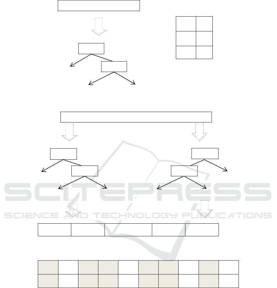
Figure 1: Example of available decision paths combination from decision tree. Courtesy of (Mitzev and Younan, 2016).
L - … L R
Figure 2: Example of decision pattern obtained as combination from presented decision tree paths. Courtesy of (Mitzev and
Younan, 2016).
R - L L R - L L L R
R L L L L - L R L L
Figure 3: Comparison coefficient is calculated by taking the count of the characters from decision pattern that coincide by
place and value and dividing it on the decision pattern length. Courtesy of (Mitzev and Younan, 2016).
4 SIMULATION RESULTS
4.1 Datasets and System Descriptions
Table 2 represents 20 selected datasets from various
domains, downloaded from the UCR database (Chen
et al., 2015). All presented datasets have less or
equal to five class labels. The specified number of
train and test time series is preliminary defined by
their authors (Chen et al., 2015). We selected the
UCR database as it appears to be very popular
among the shapelets literature and thus it became a
good ground for comparing a variety of
classification algorithms.
The experiments were provided on a regular PC
with: CPU: Intel Core i7, 2.4GHz; RAM: 8 GB. All
time series from the train dataset are normalized in
the pre-processing step according to:
L -
R L
R R
3
2
/
1
2 1
3/2
R
R
L
L
Incomin
g
time-series
3
2
/
1
2 1
3/2
Incomin
g
time-series
3
5
3
/
5
5/7
…
ICPRAM 2017 - 6th International Conference on Pattern Recognition Applications and Methods
414

X = (X - µ) / σ (2)
where µ is the average value of the time series and σ
is its standard deviation.
Table 2: Used datasets from UCR repository.
Dataset #Classes #Train/Test Length
Beef 5 30/30 470
CBF 3 30/900 128
ChlorineConcentr. 3 467/3840 166
CinC ECG torso 4 40/1380 1639
Coffee 2 28/28 286
DiatomSizeReduct. 4 16/306 345
ECGFiveDays 2 23/861 136
FaceFour 4 24/88 350
Gun_Point 2 50/150 150
Haptics 5 155/308 1092
Italy Power Demand 2 67/1029 24
Lghting2 2 60/61 637
MoteSrain 2 20/1252 84
OliveOil 4 30/30 570
SonyAIBORobotS. 2 20/601 70
SonyAIBORobotS.II 2 27/953 65
Trace 4 100/100 275
TwoLeadECG 2 23/1139 82
wafer 2 1000/6174 152
yoga 2 300/3000 426
4.2 Accuracy and Training Time
Results
To objectively assess the achieved accuracies, we
selected two reference methods– the Fast Shapelets
(FS) method (Rakthanmanon and Keogh, 2013) and
the Scalable Discovery (SD) method from
(Grabocka, Wistuba and Schmidt-Thieme, 2015).
These methods are among the fastest shapelets
training methods and maintain relatively high
accuracies. The CDP method aims to produce low
training time, especially for datasets with few class
labels, thus the SD and FS methods are good
candidates for comparison. Table 3 shows the
accuracy comparison of the three methods. The best
accuracies are highlighted. In 16 out of the 20 cases
the CDP method outperforms the reference methods
in terms of accuracy. The CDP method has more
than 10% better accuracy in 9 cases compared with
the SD method and in 8 cases compared with the FS
method.
In order to keep the training times low, we made
some improvements in the original CDP method.
The complexity of the training process for one
decision tree is in the range of O(npm
2
) per PSO
iteration, where n is the number of the train dataset
used for training, m is the average length of the time
series and p ϵ (2,4) is the number of nodes per tree.
The practice shows an average number of PSO
iterations I
PSO
to be in the range from 3 to 10. We
found that accuracy does not deteriorate if n is
reduced to up to 10 randomly selected time series.
Another improvement that was found to decrease the
training time was the reduction of the competing
random sequences into the PSO algorithm. Their
number was reduced to N
PSO
= 20, where the
candidate shapelets length varied from 3 up to N-3,
with a step of (N-6)/20. The training process is
repeated for every decision tree, where the total
number of all decision trees defines the decision
pattern length P
L.
The pattern length varies from case
to case, but usually is in the limits of up to 1000.
Thus, the overall complexity of the CDP algorithm
becomes O(Lm
2
), where L is a constant value
defined as:
L = P
L
.I
PSO
.N
PSO
.n.p (3)
In terms of the training time, the CDP method
performs relatively well keeping the training time
from several seconds up to several minutes for the
datasets shown in Table 4. The SD method produces
very low training times in the range of 0.02 up to 2
seconds. The FS method also performs well in most
of the cases, but for certain cases (“Haptics” dataset)
the training time calculations exceed one hour.
4.3 Tuning Parameters of the CDP
Method
Several CDP parameters have to be tuned in order to
produce a higher accuracy, but maintain a low
training time. The compression rate represents the
level of averaging of the neighboring values in the
time series. Compressing the signal reduces the
length of the time series and the overall complexity
of train algorithm without deteriorating much the
accuracy. Using the derivative (D) instead of the
actual signal (S) can also influence the final
accuracy. In some cases using derivative may raise
the accuracy up to 10%, in other cases it does not
influence the result or may even deteriorate the
accuracy. Another factor that greatly influences the
Concatenated Decision Paths Classification for Datasets with Small Number of Class Labels
415

Table 3: Accuracy comparisons between the Concatenated Decision Paths (CDP) method and the two reference methods:
Scalable Discovery (SD) and Fast Shapelets (FS) methods.
CDP SD FS
Dataset
Comp.
Rate
Patt.
length
S/D
Acc.,
[%]
r p
Acc.,
[%]
Acc.,
[%]
Beef 1.000 400 D 88.89 0.125 35 46.99 46.67
CBF 0.250 390 S 99.04 0.500 35 95.21 93.33
ChlorineConcentr. 1.000 450 D 73.59 0.125 15 55.41 57.01
CinC ECG torso 1.000 120 D 85.09 0.125 25 75.43 75.51
Coffee 0.250 60 S 98.81 0.250 35 96.42 92.86
DiatomSizeReduct. 0.125 540 D 90.63 0.125 15 87.79 87.91
ECGFiveDays 0.500 60 S 99.54 0.500 15 89.62 99.77
FaceFour 0.250 320 S 95.07 0.500 35 82.19 92.05
Gun_Point 0.250 66 D 98.78 0.500 25 83.55 87.33
Haptics 0.125 800 D 51.83 0.500 25 33.87 36.68
Italy Power Demand 0.500 69 S 95.62 1.000 25 89.21 93.68
Lghting2 0.250 42 S 78.14 0.500 35 77.04 72.13
MoteSrain 0.250 48 S 87.89 1.000 15 78.51 78.28
OliveOil 0.500 160 S 91.11 0.125 15 81.11 70.00
SonyAIBORobotS.. 1.000 54 S 88.08 1.000 35 77.75 68.55
SonyAIBORobotS.II 1.000 63 S 94.65 1.000 35 77.71 79.43
Trace 0.250 80 S 99.67 0.500 35 94.67 100.00
TwoLeadECG 1.000 63 S 99.85 1.000 25 88.65 92.45
wafer 1.000 81 S 99.03 0.500 35 99.19 99.64
yoga 0.250 153 S 84.16 0.250 15 79.33 68.03
Table 4: Training time comparisons between the Concatenated Decision Paths (CDP) method and the two reference
methods: Scalable Discovery (SD) and Fast Shapelets (FS) methods.
CDP SD FS
Dataset
Comp.
Rate
Patt.
length
S/D
Train
Time,
[s]
r p
Train
Time,
[s]
Train
Time,
[s]
Beef 1.000 400 D 35.3 0.125 35 0.014 116.1
CBF 0.250 390 S 7.3 0.500 35 0.015 5.5
ChlorineConcentr. 1.000 450 D 79.5 0.125 15 0.147 268.1
CinC ECG torso 1.000 120 D 132.2 0.125 25 0.330 2149.5
Coffee 0.250 60 S 2.9 0.250 35 0.039 9.5
DiatomSizeReduct. 0.125 540 D 9.3 0.125 15 0.022 11.6
ECGFiveDays 0.500 60 S 2.8 0.500 15 0.038 2.1
FaceFour 0.250 320 S 13.8 0.500 35 0.117 41.9
Gun_Point 0.250 66 D 2.1 0.500 25 0.044 3.9
Haptics 0.125 800 D 31.3 0.500 25 1.654 5684.5
Italy Power Demand 0.500 69 S 1.3 1.000 25 0.027 0.3
Lghting2 0.250 42 S 7.1 0.500 35 1.954 395.8
MoteSrain 0.250 48 S 1.2 1.000 15 0.050 0.8
OliveOil 0.500 160 S 73.7 0.125 15 0.027 79.9
SonyAIBORobotS.. 1.000 54 S 2.2 1.000 35 0.017 0.6
SonyAIBORobotS.II 1.000 63 S 2.9 1.000 35 0.023 0.7
Trace 0.250 80 S 4.9 0.500 35 0.116 79.3
TwoLeadECG 1.000 63 S 3.3 1.000 25 0.012 0.6
wafer 1.000 81 S 13.7 0.500 35 1.162 87.9
yoga 0.250 153 S 13.2 0.250 15 0.346 840.1
ICPRAM 2017 - 6th International Conference on Pattern Recognition Applications and Methods
416
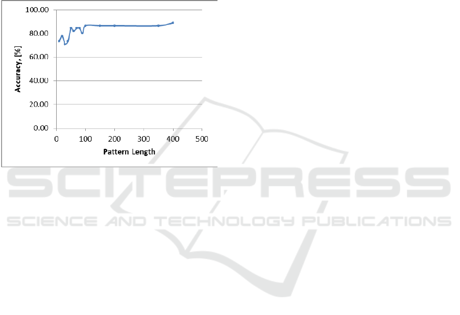
accuracy is the decision pattern length P
L
.
Increasing the P
L
generally improves the accuracy,
but it reaches a plateau as shown on Fig. 4.
The SD method has two parameters that needs to
be adjusted- the aggregation ratio (r), which
corresponds to the compression rate from CDP and
the distance threshold percent (p) that defines the
similarity threshold among the candidate shapelets.
These parameters are kept the same as defined in
accuracy report in (Grabocka, Wistuba and Schmidt-
Thieme, 2015).
Figure 4: Illustration of accuracy dependency on the
decision pattern length for “Beef” dataset.
5 CONCLUSION AND FUTURE
WORK
This work proposes an extension of the CDP method
for datasets with less than five class labels. The
initial development of the CDP method excluded the
applicability of the method for such datasets. We
have shown that because of the randomly generated
shapelets it is possible to re-train the decision trees
with the same class indexes and achieve new
decision conditions. The produced results are
compared with some of the developments in the area
that possess shortest training times: FS and SD
methods and it is shown that the CDP method
significantly outperforms these methods in terms of
accuracy.
This paper introduces some improvements to the
initially proposed CDP method in order to shorten
the training time. Training the decision tree with
less, randomly chosen train time series and reducing
the number of competitors in the PSO algorithm
helped to produce faster training times. Overall
training time of the CDP for proposed datasets is in
observable limits: varying from several seconds up
to several minutes. A future work may include
testing the CDP method with datasets with small
amount of class labels, but with very large lengths of
train time series and observe their applicability in
real industrial applications.
REFERENCES
Ye, L., Keogh, E. (2009). Time Series Shapelets: A New
Primitive for Data Mining. In: KDD’09, June 29–July
1, Paris, France, 2009.
He, Q., Dong, Z., Zhuang, F., Shang, T., Shi, Z. (2012).
Fast Time Series Classification Based on Infrequent
Shapelets. In: ICMA’12, Beijing, China, 2012.
Rakthanmanon, T., Keogh, E. (2013). Fast Shapelets: A
Scalable Algorithm for Discovering Time Series
Shapelets. In: SDM, SIAM’13, February 25- March 1,
Boston, USA, 2013.
Grabocka, J., Wistuba, M., Schmidt-Thieme, L. (2015).
Scalable Discovery of Time Series Shapelets.
arXiv:1503.03238[cs.LG], March 2015.
Mitzev, I., Younan, N. (2016). Concatenate Decision
Paths Classification for Time Series Shapelets. In:
CMCA’16, January 2-3, Zurich, Switzerland, 2016.
Mitzev, I., Younan, N. (2015). Time Series Shapelets:
Training Time Improvement Based on Particle Swarm
Optimization. IJMLC, vol. 5, August 2015
Chen, Y., Keogh, E., Bing, H., Begum, N., Bagnall, A.,
Mueen, A., Batista, G. (2015). The UCR Time Series
Classification Archive. [online]. Available at:
http://www.cs.ucr.edu/~eamonn/time_series_data/.
Grabocka, J., Wistuba, M., Schmidt-Thieme, L. (2015).
Scalable Discovery of Time-Series Shapelets. [online].
Available at: www.dropbox.com/sh/btiee2pyn6a989q/
AACDfzkkpdYPmgw7pgTgUoeYa
Keogh, E., Rakthanmanon, T. (2013). Fast Shapelets: A
scalable Algorithm for Discovering Time Series
Shapelets. [online]. Available at:
http://alumni.cs.ucr.edu/~rakthant/FastShapelet
Concatenated Decision Paths Classification for Datasets with Small Number of Class Labels
417
