New Scenario-based Stochastic Programming Problem for Long-term

Allocation of Renewable Distributed Generations

Ikki Tanaka

and Hiromitsu Ohmori

Graduate School of Science and Technology, Keio University, Kanagawa, Japan

Department of System Design Engineering, Keio University, Kanagawa, Japan

Keywords:

Stochastic Optimization, Power Systems, Renewable Energy Sources, Distributed Generations, Expansion

Planning.

Abstract:

Large installation of distributed generations (DGs) of renewable energy sources (RESs) on distribution net-

work has been one of the challenging tasks in the last decade. According to the installation strategy of Japan,

long-term visions for high penetration of RESs have been announced. However, speciﬁc installation plans have

not been discussed and determined. In this paper, for supporting the decision-making of the investors, a new

scenario-based two-stage stochastic programming problem for long-term allocation of DGs is proposed. This

problem minimizes the total system cost under the power system constraints in consideration of incentives to

promote DG installation. At the ﬁrst stage, before realizations (scenarios) of the random variables are known,

DGs’ investment variables are determined. At the second stage, after scenarios become known, operation and

maintenance variables that depend on scenarios are solved. Furthermore, a new scenario generation procedure

with clustering algorithm is developed. This method generates many scenarios by using historical data. The

uncertainties of demand, wind power, and photovoltaic (PV) are represented as scenarios, which are used in

the stochastic problem. The proposed model is tested on a 34 bus radial distribution network. The results

provide the optimal long-term investment of DGs and substantiate the effectiveness of DGs.

1 INTRODUCTION

1.1 Background

Large penetration of RESs-based DGs in distribution

network implies that distribution companies (DIS-

COs) need to deal with the intermittent nature of

RES such as wind speed and solar radiation in order

to maintain the demand-and-supply balance contin-

uously, and accommodate expected demand growth

over the planning horizon (Eftekharnejad et al.,

2013). DGs refer to small-scale energy generations

and are most generally used to guarantee that suf-

ﬁcient energy is available to meet peak demand.

Distributed generation planning (DGP), which de-

termines the optimal siting, sizing, and timing, is

modeled to tackle above problem. The objective of

DGP is to ensure that the reliable power supply to

the consumers is achieved at a lowest possible cost.

DGP plays an important role as a strategic-level plan-

ning in modern power system planning. Commonly

used approaches to solve the DGP are: sensitivity

analysis-based approaches, mixed-integer linear pro-

gramming, and nonlinear programming. However,

the above methods can not fully handle the uncer-

tainties. Consequently, stochastic programming and

metaheuristic-based approaches have been used these

days, to consider the uncertainties at the energy plan-

ning (Payasi et al., 2011; Jordehi, 2016).

1.2 Related Work

Much attention has been paid to solving several

stochastic problems for one-type capacity planning.

For multi-resource type, the scenario-based tech-

niques also have been proposed to consider various

uncertainties (Huang and Ahmed, 2009; Baringo and

Conejo, 2013b; Munoz et al., 2016).

In power system planning on transmission and

distribution network, many approaches have been

developed considering some RESs, energy conver-

sion and transmission, and the uncertainties that are

caused by demand, pricing, and intermittent renew-

ables (Verderameet al., 2010). An energy planning in

individual large energy consumers was formulated as

a mixed integer linear programming model by using

Tanaka I. and Ohmori H.

New Scenario-based Stochastic Programming Problem for Long-term Allocation of Renewable Distributed Generations.

DOI: 10.5220/0006189900960107

In Proceedings of the 6th International Conference on Operations Research and Enterprise Systems (ICORES 2017), pages 96-107

ISBN: 978-989-758-218-9

fuzzy parameters in (Mavrotas et al., 2003). (Atwa

et al., 2010) proposed a probabilistic mixed integer

nonlinear problem for distribution system planning.

Several studies related to stochastic optimization

of DGP have been proposed. In (Fu et al., 2015),

a chance-constrained stochastic programming model

was formulated for managing the uncertainty of PV,

which was solved by an algorithm combining the

multi-objective particle swarm optimization with sup-

port vector machines. (Abdelaziz et al., 2015) pro-

vided an energy loss minimization problem which de-

termines the optimal location of RES-based DGs and

the location and daily schedule of dispatch-able DG.

In the problem, the uncertainties between wind power,

PV and demand were considered using the diago-

nal band Copula and sequential Monte Carlo method.

In (Saif et al., 2013), the uncertainties of wind en-

ergy, PV, and energystorage system were produced as

chronological ones for a two-layer simulation-based

allocation problem. In (Pereira et al., 2016), the al-

location problem of VAR compensator and DG was

formulated as a mixed-integer nonlinear problem and

solved by using meta-heuristic algorithms.

A two-stage architecture is commonly used in

stochastic programming approaches. At the ﬁrst

stage, DGs’ investment variables are determined be-

fore realizations of random variables are known, i.e.,

scenarios. At the second stage, after scenarios be-

come known, operation and maintenance variables

which depend on scenarios are solved.

(Carvalho et al., 1997) modeled a two-stage

scheme problem of distribution network expansion

planning under uncertainty in order to minimize an

expected cost along the horizon and solved by the pro-

posed hedging algorithm in an evolutionary approach

to deal with scenario representation efﬁciently. In

(Krukanont and Tezuka, 2007), a two-stage stochas-

tic programming for capacity expansion planning was

provided in a power system of Japan. This model

includes the uncertainties of the demand, carbon tax

rate, operational availability. In (Wang et al., 2014), a

two-stage robust optimization-based model consider-

ing uncertainties of DG outputs and demand was pro-

vided for the optimal allocation of DGs and micro-

turbine. (Montoya-Bueno et al., 2015) proposed a

stochastic two-stage multi period mixed-integer lin-

ear programming model of renewable DG allocation

problem considering the uncertainties affected by de-

mand and renewable energy production.

As an allocation problem of energy storage sys-

tem (ESS), (Nick et al., 2014) formulated the op-

timal allocation problem as a two-stage stochas-

tic mixed-integer second-order cone programming

(SOCP) model. In (Nick et al., 2015), SOCP prob-

lem of ESS allocation was solved by using alterna-

tive direction method of multipliers. In (Asensio

et al., 2016a; Asensio et al., 2016b), the allocation

problem of DGs and energy storage was formulated

as a stochastic programming model for maximizing

the net social beneﬁt taking account of demand re-

sponse. Since the cost of ESS is very expensive and

ESS seems not to be efﬁcient at this stage, ESS is ex-

cluded from consideration in this paper.

In solving the two-stage stochastic programming,

an effective methodology to create proper scenarios

must be needed to represent various uncertainties be-

cause it is very difﬁcult to realistically obtain all of the

information about the uncertainty and computation-

ally incorporate it into the model. In case some proba-

bility distributions are analytically estimated and used

instead, the problem commonly becomes very com-

plexed, even if the problem is small. Hence, when

the partial information of the uncertainty is available,

the stochastic programing model normally needs to be

solved using scenarios. There exist many techniques

of scenario generation (Dupaˇcov´a et al., 2000). The

uncertainty modeling such as demand and wind speed

were developed to create scenarios in (Baringo and

Conejo, 2011). The proposed method uses dura-

tion curves which is approximated by some demand

blocks. (Baringo and Conejo, 2013a) performed the

scenario reduction by using K-means clustering algo-

rithm to arrange the historical scenarios of demand

and wind into clusters according to the similarities.

(Sadeghi and Kalantar, 2014) used Monte Carlo sim-

ulation and probability generation load matrix for ob-

taining the uncertainty of fuel and electricity price,

DG outputs, and load. In (Mazidi et al., 2014), the

Latin hypercube sampling was used to prepare sce-

narios of RESs. In (Seljom and Tomasgard, 2015), an

iterative-random-sampling-based scenario generation

algorithm was developed. They evaluated whether

the number of scenarios is enough to obtain reliable

results. In (Nojavan and allah Aalami, 2015), the

normal distribution and the Weibull distribution were

used for generating the scenarios of electric price, de-

mand, and meteorological data. The created scenarios

were reduced by the fast forward selection based on

Kantorovich distance approach. In (Montoya-Bueno

et al., 2016), a probability density function-based sce-

nario generation method was proposed for the alloca-

tion problem of wind power and PV.

1.3 Contribution

Most of scenario generation have not considered

the correlation between the uncertainties (e.g., de-

mand and solar radiation) and usually the uncertainty

New Scenario-based Stochastic Programming Problem for Long-term Allocation of Renewable Distributed Generations

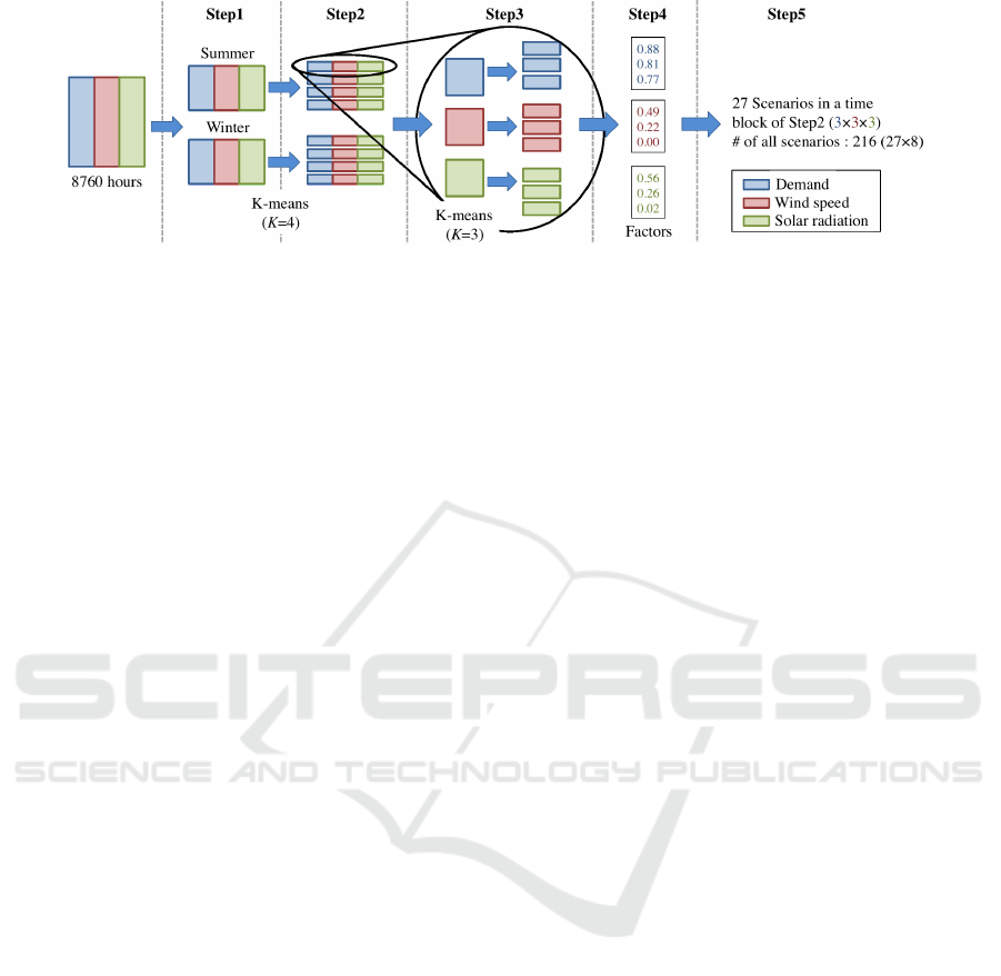
Figure 1: Outline of scenario generation. This ﬁgure shows the procedure focused on a block in Step 2.

separations to the levels have been made manually

(Baringo and Conejo, 2011; Montoya-Bueno et al.,

2016). It is necessary, however, to create scenarios

automatically in consideration of the correlations for

appropriate scenarios based on data. In optimization

problem mentioned above, many researches of opti-

mal DG allocation problem that takes into account the

uncertainties have been performed. Most of the stud-

ies have considered only one-year’s allocation and

daily/annual system operation. Realistically, in order

to accomplish the optimal system operation in multi-

period, obtaining the long-term optimal siting, sizing,

and timing is required. Hence, this study provides the

two main contributions as follows.

• A new scenario generation method with K-means

is proposed to create scenario-levels automati-

cally by using similarity measure. This procedure

uses historical data and can be implemented read-

ily. If K-means algorithm is simply applied to

the available data, it is not possible to take into

account the correlation between demand and me-

teorological data or seasonal characteristics (e.g.,

summer and winter). Hence, in the proposed ap-

proach K-means clustering is utilized in stages by

focusing on demand and seasons. Many scenarios

of demand, wind speed, and solar radiation are

generated and appropriate probabilities of each

scenario are calculated (not equal-probability) by

use of divided time blocks.

• A new long-term allocation problem of RES-

based DGs is proposed. This model is formu-

lated as a two-stage stochastic programmingprob-

lem with the objective of minimizing the total

system cost. In the proposed model, some de-

vices and constraints are integrated for improv-

ing distribution system (i.e., limitation of reverse

power ﬂow, generation of DG considering lag-

ging/leading power factor, capacitor bank (CB)).

Furthermore, the carbon emission costs and in-

centives are considered from the point of view

of international trends and economics because the

problems of carbon emissions are actively dis-

cussed at the Conference of the Parties to the UN-

FCCC to achieve a clean environment and the

government generally, in order to reach high re-

newable penetration levels, subsidizes the DIS-

COs that invest RES to their distribution system.

1.4 Paper Organization

The reminder of this paper is organized as follows. In

Section 2, the details of the proposed scenario gen-

eration procedure is described. Section 3 provides

the stochastic programming model. The results of the

numerical simulations are presented and discussed in

Section 4. Finally, the paper is concluded providing

some insights and summaries in Section 5.

2 SCENARIO GENERATION

This Section describes the proposed scenario gener-

ation method that applies K-means to historical data

(i.e. load, wind speed, solar radiation) in stages. The

goal is to obtain the scenario levels of demand, elec-

tricity price, wind speed, and solar radiation for creat-

ing speciﬁc scenarios. The role of K-means is to clas-

sify a original dataset into a certain number of clus-

ters K. The centroid of each cluster is the mean value

of the data allocated to each cluster. The algorithm

is based on the iterative ﬁtting process as following

steps:

1. Select the number of clusters K according to

the speciﬁc problem. Randomly place K points,

which represent the initial cluster centroids, into

the space represented by the clustered dataset.

2. Assign each data to the closest centroid base on

the distances.

3. When all data have been assigned, recalculate the

new cluster centroids using data allocated to each

cluster.

4. Repeat Steps 2 and 3 iteratively until there are no

changes in any mean, i.e. the centroids no longer

ICORES 2017 - 6th International Conference on Operations Research and Enterprise Systems

move. As a result, the clustered dataset is sepa-

rated into groups minimizing an objective func-

tion, in this paper a quadratic distance is used.

Historical data need to be available for scenario cre-

ation, i.e. hourly demand, wind speed, solar radiation,

and electricity price data for the 8760 hours of the

year. Figure 1 shows the overview of the proposed

scenario generation. The steps are described below:

Step 1) Normalize data into the [0.0,1.0] interval by

dividing by the maximum value of each feature

and simultaneously separate into two seasons :

summer (April-September) and winter (October-

March). Each seasonal group consists of 4380

hours block.

Step 2) Apply K-means (the number of clusters K =

4) to only the demand in each seasonal groups cre-

ated in Step 1 and allocate each data into four

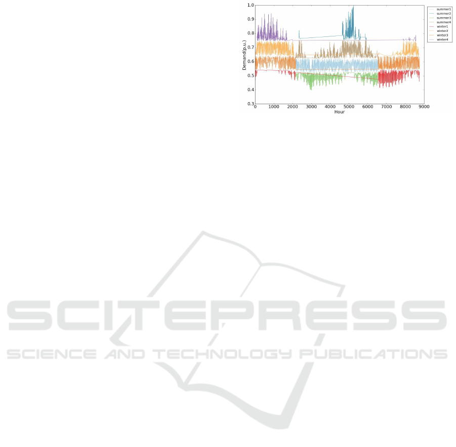
groups. Figure 2 shows the clusters of the de-

mand. Moreover, wind speed, solar radiation and

price indexed to each demand data are also allo-

cated to the same clusters of the demand. Each

divided group is deﬁned as a time block b, which

is related to the representativesof demand clusters

(e.g., peak-load of summer, middle-load of sum-

mer, low-load of winter). Total of the number of

hours in time block b is represented as N

hours

Step 3) Apply K-means (K = 3) again into the de-

mand, wind speed, and solar radiation of the data

group created in Step 2 respectively and 9 data

groups are created per one block. Step 3-5 in Fig.

1 focus on the ﬂow of the one of the data blocks

in Step 2.

Step 4) The mean values of each data block in Step

3 are used as a block representative to create the

factors of demand, wind speed, and solar radia-

tion. Note that the price levels are determined

by the mean values of the price within each de-

mand block. Renewable production models in

(Eduardo, 1994) and (Atwa et al., 2010) are used

in this paper so that renewable observation data

are transformed into power output (i.e., wind gen-

eration factor and PV generation factor)

Step 5) Considering the combination of each factor

made in Step 4, 27 scenarios are obtained for

each time block. Therefore, 216 scenarios are

obtained as the total number of scenarios. The

probabilities of the factors within each time block,

load

b,s

, Pr

b,s

, Pr

b,s

,are deﬁned by the ratio of the

number of hours of the blocks divided in Step3

to the corresponding block in Step2, i.e., N

hours

Hence, the scenario probabilities Pr

b,s

are calcu-

Figure 2: The clusters of demand in Step 2 (time blocks).

lated as:

b,s

= Pr

load

b,s

× Pr

b,s

× Pr

b,s

Note that the time block b represents the demand pe-

riods related to season (e.g., high-demand in summer,

low-demand in winter) and the index s represents the

scenarios in the time block b (e.g., (high demand,

large wind, large PV), (low-demand, middle wind,

small PV)).

3 OPTIMAL LONG-TERM

ALLOCATION PROBLEM OF

DISTRIBUTED GENERATION

Two-stage stochastic linear programming is used as

a formulation of the long-term allocation problem of

DGs. The model uses the scenarios and provides the

optimal siting, sizing, and timing of RES-based DGs

to be installed (wind power and PV). The nomencla-

ture related to the problem formulation described in

Appendix.

3.1 Objective Function

This model minimizes the total system cost consisting

of the investment cost π

inv

and operation & mainte-

nance cost in consideration of the incentive µ

inc

. The

expected value of the O&M cost in year t is shown as:

∑

b∈Ω

hours

t,b

∑

s∈Ω

t,b

t,b,s

,t ∈ Ω

(1)

where, Ω

is the set of time blocks in year t, N

hours

t,b

is the total hours of time block b in t, Ω

t,b

is the set

of the scenarios in t and b, Pr

t,b,s

is the probability of

the scenario s in t and b, and π

t,b,s

is the O&M cost

per unit time in t, b, and s. In this paper, it is assumed

that the time blocks and scenarios are the same every

year,

Ω

= Ω

, N

hours

t,b

= N

hours

, Ω

t,b

= Ω

, Pr

t,b,s

= Pr

b,s

New Scenario-based Stochastic Programming Problem for Long-term Allocation of Renewable Distributed Generations

because, in the same region, the trend of the demand

proﬁle and the average of the weather data are consid-

ered not to change signiﬁcantly. It is important to note

that the operational environment of the power sys-

tem is different in each year since the time-dependent

parameters exist, such as demand growth factor, dis-

count rate, and price increasing factor, although the

scenarios do not change.

Therefore, the aim of the model is minimizing the

total system cost over the planning horizon T:

Minimize:

∑

t∈Ω

inv

∑

b∈Ω

hours

∑

s∈Ω

b,s

t,b,s

−

∑

t∈Ω

inc

(2)

where α

(1+d)

is the present value factor.

3.1.1 Investment Costs

The following equations show the investment costs of

the substation, wind turbine, PV, and CB. The costs

are, respectively, annualized by using the interest rate

and lifetime of the devices. Therefore, the previous

year’s investment cost is added to the next one except

for the ﬁrst year.

inv

∑

n∈Ω

anu

SS,n

∑

n∈Ω

(π

anu

PV,n

+ π

anu

WD,n

+ π

anu

CB,n

) + π

inv

t−1

;t > 1,

(3)

inv

∑

n∈Ω

anu

SS,n

∑

n∈Ω

(π

anu

PV,n

+ π

anu

WD,n

+ π

anu

CB,n

) ;t = 1,

(4)

anu

inv

i(1+ i)

(1+ i)

− 1

, (5)

anu

inv

i(1+ i)

(1+ i)

− 1

, (6)

anu

inv

i(1+ i)

(1+ i)

− 1

, (7)

anu

inv

i(1+ i)

(1+ i)

− 1

. (8)

3.1.2 Operation and Maintenance Costs

O&M costs are shown in the following equations. To-

tal O&M cost includes the power loss cost, unserved

energy cost, purchased energy cost, O&M cost of

DGs and CB, and CO

emission cost.

t,b,s

= π

loss

t,b,s

+ π

ENS

t,b,s

+ π

t,b,s

+ π

new

t,b,s

+ π

t,b,s

+ π

emi

t,b,s

(9)

loss

t,b,s

= π

loss

∑

n,m∈Ω

base

n,m

sqr,n,m

t,b,s

, (10)

ENS

t,b,s

= π

ENS

∑

n∈Ω

base

ENS,n

t,b,s

, (11)

t,b,s

= π

b,s

∑

n∈Ω

base

SS,n

t,b,s

, (12)

new

t,b,s

= S

base

∑

n∈Ω

(π

PV,n

t,b,s

+ π

WD,n

t,b,s

), (13)

t,b,s

= S

base

∑

n∈Ω

CB,n

t,b,s

, (14)

emi

t,b,s

= π

emi,SS

t,b,s

+ π

emi,DG

t,b,s

, (15)

emi,SS

t,b,s

= η

emi

base

∑

n∈Ω

emi

SS,n

t,b,s

, (16)

emi,DG

t,b,s

= η

emi

base

∑

n∈Ω



emi

WD,n

t,b,s

+ν

emi

PV,n

t,b,s



(17)

3.1.3 Incentive

Incentive will be paid for the new investment of DGs

by using the subsidy rare.

inc

= α

∑

n∈Ω



sub

inv

WD,n

+ γ

sub

inv

PV,n



(18)

3.2 Constraints

3.2.1 Power Balance Constraints

The following constraints describe the active and re-

active power balance of the load and substation buses.

It should be mentioned that the scenario of demand,

load

b,s

, is used by multiplying the peak load of each

bus.

∑

n,m∈Ω



n,m

t,b,s

− r

n,m

sqr,n,m

t,b,s



−

∑

m,n∈Ω



m,n

t,b,s



+ P

ENS,m

t,b,s

+ P

WD,m

t,b,s

+ P

PV,m

t,b,s

= η

load

b,s

load,m

(19)

∑

n,m∈Ω



n,m

t,b,s

− r

n,m

sqr,n,m

t,b,s



−

∑

m,n∈Ω



m,n

t,b,s



SS,m

t,b,s

= η

load

b,s

load,m

(20)

∑

n,m∈Ω



n,m

t,b,s

− x

n,m

sqr,n,m

t,b,s



−

∑

m,n∈Ω



m,n

t,b,s



+ Q

WD,m

t,b,s

+ Q

PV,m

t,b,s

+ Q

CB,m

t,b,s

= η

load

b,s

load,m

(21)

∑

n,m∈Ω



n,m

t,b,s

− x

n,m

sqr,n,m

t,b,s



−

∑

m,n∈Ω



m,n

t,b,s



SS,m

t,b,s

= η

load

b,s

load,m

(22)

ICORES 2017 - 6th International Conference on Operations Research and Enterprise Systems

100

3.2.2 Voltage and Current Equations

The nodal voltage equation and power ﬂow equation

are shown as follows:

sqr,m

t,b,s

− 2(r

m,n

t,b,s

+ x

m,n

t,b,s

)

+|z

m,n

sqr,m,n

t,b,s

−V

sqr,n

t,b,s

= 0,

(23)

sqr,m

t,b,s

sqr,m,n

t,b,s

= P

m,n

t,b,s

+ Q

m,n

t,b,s

. (24)

To transform the non-linear equation (24) into the

linear equation, the piecewise linear approximation

described in (Zou et al., 2010) is used in this paper.

The equation is linearized as follows:

nom

sqr,m,n

t,b,s

∑

h∈Ω



m,n,h

t,b,s

∆P

m,n,h

t,b,s



∑

h∈Ω



m,n,h

t,b,s

∆Q

m,n,h

t,b,s



(25)

m,n

t,b,s

= P

+,m,n

t,b,s

− P

−,m,n

t,b,s

, (26)

m,n

t,b,s

= Q

+,m,n

t,b,s

− Q

−,m,n

t,b,s

, (27)

P+,m,n

t,b,s

+ X

P−,m,n

t,b,s

≤ 1, (28)

Q+,m,n

t,b,s

+ X

Q−,m,n

t,b,s

≤ 1. (29)

+,m,n

t,b,s

+ P

−,m,n

t,b,s

∑

h∈Ω

∆P

m,n,h

t,b,s

, (30)

+,m,n

t,b,s

+ Q

−,m,n

t,b,s

∑

h∈Ω

∆Q

m,n,h

t,b,s

, (31)

0 ≤ ∆P

m,n,h

t,b,s

≤ ∆S

m,n,h

t,b,s

, (32)

0 ≤ ∆Q

m,n,h

t,b,s

≤ ∆S

m,n,h

t,b,s

, (33)

m,n,h

t,b,s

= (2h− 1)∆S

m,n,h

t,b,s

, (34)

∆S

m,n,h

t,b,s

nom

m,n

. (35)

3.2.3 Current, Voltage, and Power Limits

The current on branches, voltage of buses, and power

ﬂow on branches should be limited in the allowable

range:

0 ≤ V

nom

sqr,m,n

t,b,s

≤

m,n

, (36)

≤ V

sqr,m

t,b,s

≤ V

, (37)

0 ≤ P

+,m,n

t,b,s

≤ V

nom

m,n

P+,m,n

t,b,s

(38)

0 ≤ P

−,m,n

t,b,s

≤

rev,m,n

P−,m,n

t,b,s

, (39)

0 ≤ Q

+,m,n

t,b,s

≤ V

nom

m,n

Q+,m,n

t,b,s

, (40)

0 ≤ Q

−,m,n

t,b,s

≤ V

nom

m,n

Q−,m,n

t,b,s

. (41)

3.2.4 Maximum DG Size Limits

The following constraint deﬁnes the maximum DG

installation capacity of each bus:

∑

t∈Ω

(

WD,n

+ P

PV,n

) ≤ P

node

. (42)

3.2.5 DG & CB Generation Limits

0 ≤ P

WD,n

t,b,s

≤ η

b,s

avl,WD,n

, (43)

0 ≤ P

PV,n

t,b,s

≤ η

b,s

avl,PV,n

, (44)

0 ≤ Q

CB,n

t,b,s

≤ Q

avl,CB,n

. (45)

Constraints (43) – (45) express the minimum and

maximum generation of DGs and CB. Note that the

scenarios of the wind power and PV, i.e., produc-

tion factors η

b,s

and η

b,s

, are used by multiplying

the maximum available output of each installed DG.

The following constraints show the maximum avail-

able output in each year:

avl,WD,n

WD,n

;t = 1, (46)

avl,WD,n

WD,n

+ P

avl,WD,n

t−1

;t > 1 (47)

avl,PV,n

= P

PV,n

;t = 1, (48)

avl,PV,n

PV,n

+ P

avl,PV,n

t−1

;t > 1, (49)

avl,CB,n

CB,n

;t = 1, (50)

avl,CB,n

CB,n

+ Q

avl,CB,n

t−1

;t > 1. (51)

The number of installations of DG and CB in each

bus is limited as,

∑

t∈Ω

WD,n

≤

, (52)

∑

t∈Ω

PV,n

≤

, (53)

∑

t∈Ω

CB,n

≤

. (54)

The constraints of the reactive power produced by

DGs are expressed by using leading/lagging power

factor:

−tan(cos

−1

(λ

lead

))P

WD,n

t,b,s

≤ Q

WD,n

t,b,s

≤tan(cos

−1

(λ

lag

))P

WD,n

t,b,s

(55)

−tan(cos

−1

(λ

lead

))P

PV,n

t,b,s

≤ Q

PV,n

t,b,s

≤tan(cos

−1

(λ

lag

))P

PV,n

t,b,s

(56)

New Scenario-based Stochastic Programming Problem for Long-term Allocation of Renewable Distributed Generations

101

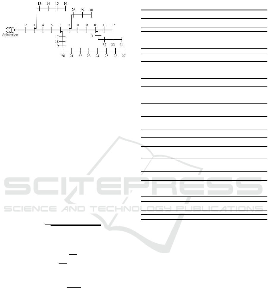
Figure 3: Distribution system conﬁguration.

3.2.6 Investment Limits

The following constraints refer to the annualized and

actual investment cost limits considering the lifetime.

inv

≤ π

bgt

inv

, (57)

∑

t∈Ω

[

∑

n∈Ω

inv

SS,n

∑

n∈Ω

(π

inv

PV,n

+π

inv

WD,n

+ π

inv

CB,n

)] ≤ π

bgt

(58)

3.2.7 Energy Not Supplied Limits

The unserved power must be less than the demand:

0 ≤ P

ENS,n

t,b,s

≤ η

load

b,s

load,n

, (59)

0 ≤ Q

ENS,n

t,b,s

≤ η

load

b,s

load,n

. (60)

3.2.8 Substation Limits

The following constraints show the generation limit

of the substation.

SS,n

t,b,s

≤

avl,SS,n

1+ tan(cos

−1

(λ

))

, (61)

0 ≤ Q

SS,n

t,b,s

≤ tan(cos

−1

(λ

))P

SS,n

t,b,s

, (62)

avl,SS,n

= S

SS,n

+ S

new,n

, (63)

new,n

= X

SS,n

;t = 1, (64)

new,n

= X

SS,n

+ S

new,n

t−1

;t > 1. (65)

The substation expansion is allowed up to the

maximum power:

new,n

≤

new,n

. (66)

4 NUMERICAL SIMULATION

4.1 Distribution System

The 34-bus three-phase radial feeder, shown in Figure

3, is used to test the proposed scenario generation and

allocation problem. The system has 1 substation and

33 buses with/without load. Details of the network

are given in (Chis et al., 1997).

Table 1: Simulation parameters.

Total peak load

power

5.45 (MVA)

Initial available

substation power

5.50 (MVA)

Capacity of wind

turbine and PV

100, 2.5 (kW) Capacity of CB 100 (kVar)

Base power 10 (MVA) Base voltage 11 (kV)

Maximum power

that can be

installed at each

bus

250 (kW)

Maximum numbers

of wind turbine, PV

modules, and CB

2, 85, 5

Thermal capacity 6.5 (MVA) Substation voltage 1.04 (p.u.)

Annual demand

growth

2 (%)

Price increasing

factor

1 (%)

Minimum/

maximum limits

of voltage

magnitude

±5% (0.95 and

1.05 p.u.)

Number of

segments used in

the piecewise

linearization

Increasing factor

of emission cost

2 (%) Lifetime of devices 20 (years)

Investment cost of

transformer, wind

turbine, PV

module, and CB

20000,125155,

3455,38500(e)

O&M costs of wind

turbine, PV, and CB

0.0079,0.0064

(e/kWh)

,0.003(e/kVarh)

Subsidy rate of

wind turbine and

10, 5 (%)

Power factor at the

substation

0.9013

Discount rate 12.5 (%)

Lagging/leading

power factor of

DGs

0.9013, 0.0

Interest rate 8 (%)

Cost of CO

emission

30 (e/tCO

)

Investment budget

per year

350000 (e)

Emission rate of

purchased energy

0.55

(tCO

/MWh)

Investment budget

throughout the life

cycle of devices

5500000 (e)

Emission rate of

wind turbine and

0.25 and 0.26

(tCO

/MWh)

Cost of not

supplied energy

15000

(e/MWh)

Maximum

expansion of the

substation

5 (MVA)

Candidate buses of

wind turbines

13-16, 21-27

Candidate buses of

11, 12, 24-27,

31-34

Table 2: Model information.

Number of continuous variables 2,810,473

Number of general integer variables 444,960

Number of binary variables 570,240

Number of linear constraints 4,578,985

Number of non zero coefﬁcients 14,070,169

4.2 Data and Parameters

The simulation parameters are shown in Table 1. Ac-

tual load data of Tokyo Electric Power Company

(TEPCO) are used as demand. The wind speed

and solar radiation are the meteorological observation

data of Miyakojima Island in Japan from Jan. 1, 2015

to Dec. 31, 2015. A twenty-year period is used as a

planning horizon. Demand, wind, PV, and price lev-

els are described in Table 3. The problem is solved

using Gurobi 6.5.0 (Gurobi 6.5.0, 2016) on a Linux-

based computer with 4-core Intel

Core i7-4770 at

3.4 GHz and 24 GB of RAM. The information about

the overall model is described in Table 2.

4.3 Simulation Cases

The following three cases are consided:

Case A: The investment is only allowed for the ex-

pansion of the substation, i.e., the right-hand side

of Eq. (42) is zero.

ICORES 2017 - 6th International Conference on Operations Research and Enterprise Systems

102

Table 3: Scenario factors of each time block. The values in

parentheses represent the factor’s probabilities.

Time

Blocks

Hours

Price

(e/MWh)

Demand

factors

Wind factors PV factors

97.63 0.61 (0.328) 0.41 (0.370) 0.65 (0.163)

1 1370 98.04 0.58 (0.328) 0.16 (0.207) 0.29 (0.602)

98.28 0.54 (0.344) 0.00 (0.423) 0.02 (0.235)

103.08 0.93 (0.433) 0.41 (0.329) 0.68 (0.321)

2 420 103.01 0.84 (0.236) 0.20 (0.443) 0.41 (0.371)

102.44 0.78 (0.331) 0.00 (0.229) 0.06 (0.307)

97.84 0.51 (0.212) 1.00 (0.423) 0.62 (0.910)

3 1316 97.68 0.48 (0.444) 0.23 (0.572) 0.28 (0.066)

97.19 0.44 (0.344) 0.00 (0.005) 0.01 (0.024)

100.60 0.73 (0.381) 0.92 (0.428) 0.68 (0.451)

4 1286 99.20 0.68 (0.171) 0.28 (0.022) 0.37 (0.271)

98.26 0.64 (0.448) 0.00 (0.550) 0.05 (0.278)

94.15 0.52 (0.245) 0.69 (0.109) 0.59 (0.070)

5 960 94.15 0.48 (0.453) 0.33 (0.529) 0.29 (0.060)

94.15 0.45 (0.302) 0.01 (0.361) 0.01 (0.870)

94.15 0.73 (0.324) 0.46 (0.236) 0.58 (0.155)

6 1205 94.15 0.69 (0.381) 0.24 (0.441) 0.28 (0.207)

94.15 0.66 (0.295) 0.00 (0.323) 0.03 (0.638)

94.15 0.62 (0.370) 0.50 (0.248) 0.57 (0.675)

7 1590 94.15 0.59 (0.304) 0.25 (0.354) 0.27 (0.143)

94.15 0.56 (0.326) 0.00 (0.397) 0.01 (0.182)

94.15 0.88 (0.502) 0.49 (0.323) 0.56 (0.726)

8 613 94.15 0.81 (0.168) 0.22 (0.393) 0.26 (0.096)

94.15 0.77 (0.330) 0.00 (0.284) 0.02 (0.178)

Table 4: O&M costs (e).

Cases A B C

Losses cost 1,163,844 1,012,212 786,011

Not supplied energy cost 45,320 67,221 4,937

Purchased energy cost 24,975,772 22,841,032 16,196,578

DG O&M cost 0 141,731 572,780

Capacitor bank cost 218,980 193,093 134,986

Emission cost 4,567,235 4,196,637 3,043,670

O&M system cost 30,971,152 28,451,927 20,738,962

Table 5: Total system costs (e).

Cases A B C

O&M system cost 30,971,152 28,451,927 20,738,962

Investment costs 413,085 2,228,716 8,369,486

Incentive 0 185,179 697,443

Total costs 31,384,236 30,495,464 28,411,005

Computational time 25262 s 277680 s 34693 s

Case B: All the constraints are considered.

Case C: Case B without investment constraints (57)

and (58).

4.4 Results and Discussions

Tables 4 and 5 show the O&M costs and total system

costs. Optimal location, sizing, and timing are shown

in Tables 6 and 7. The installation of DGs plays an

important role to reduce the total system cost despite

the fact that the investment costs are increasing. A

signiﬁcant contribution is that it drastically reduces

the O&M costs (see Table 4). This is one of the gen-

eral beneﬁts of DG installment. From Table 4, the

greatest cost savings occur in the emission cost be-

cause the emission rate of the purchased energy at

the substation is two times higher than that of the

DGs. Moreover, the losses cost and purchased energy

cost are reduced since most DGs are allocated around

the terminal buses of radial distribution system. As

Table 6: Optimal location and timing (bus).

Cases

A B C

Years SUB CB SUB WD PV CB SUB WD PV CB

12 21

22 23

25 26

27 33

24 25

24 26

27 33

11 12

21 22

23 25

26 32

13 14

15 21

22 23

24 25

26 27

11 12

24 25

26 27

31 32

33 34

11 21

22 23

25 26

2 11 14

3 24 24

4 16

5 1 16

6 1 1

7 1 23

8 21

9 21 24

12 27

13 21 31 1 21 31 21 31

14 21

23 25

11 23

12 21

11 14

22 26

22 31

11 21

25 33

11 15

21 22

24 31

11 21

22 24

17 13 22

22 25

14 15

22 31

12 13

24 32

11 13

13 14

21 31

13 24

20 16

15 22

31 32

Table 7: Optimal sizing (kW).

Cases

A B C

Years SUB CB SUB WD PV CB SUB WD PV CB

1 800 600 262.5 800 1500 1875 600

2 100 100

3 100 100

4 100

5 1000 100

6 1000 1000

7 1000 100

8 100

9 100 100

12 100

13 200 1000 200 200

14 500 300 1000 300

15 400 400 400

16 400 500 400

17 400 400 500

18 500 100 400

19 500 500

20 100 400

Total 2000 4100 2000 600 262.5 3000 2000 1800 1875 3900

shown in Table 6, the DGs allow the substation ex-

pansion to defer. However, the results imply that the

expansion is not inevitable due to the intermittent na-

ture of renewable DGs and the demand growth (see

Table 7).

The O&M cost of CB decreases even if the num-

ber of CB increases (see Tables 4 and 7), imply-

ing that CB co-exists well with the large amount of

the installed DGs. Without the budget constraints,

nearly the same amount of wind turbine and PV are

installed. However, in the consideration of the bud-

gets, the wind power to be installed is larger than PV

because it is affected by the high subsidy rate of wind.

In the same way, the simulations without the in-

centive were tested, i.e., the incentives of wind en-

ergy and PV are 0. The O&M and total system costs

are shown in Tables 8 and 9. Tables 5 and 9 indi-

New Scenario-based Stochastic Programming Problem for Long-term Allocation of Renewable Distributed Generations

103

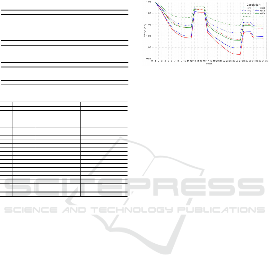
Table 8: O&M costs (e).

Cases A B C

Losses cost 1,163,844 1,000,584 795,689

Not supplied energy cost 45,320 71,244 359

Purchased energy cost 24,975,772 22,808,383 16,558,486

DG O&M cost 0 133,506 537,774

Capacitor bank cost 218,980 196,581 133,903

Emission cost 4,567,235 4,191,123 3,105,423

O&M system cost 30,971,152 28,401,420 21,131,633

Table 9: Total system costs (e).

Cases A B C

O&M system cost 30,971,152 28,401,420 21,131,633

Investment costs 413,085 2,262,126 7,914,809

Incentive 0 0 0

Total costs 31,384,236 30,663,546 29,046,443

Table 10: Optimal sizing under no incentive (kW).

Cases

A B C

Years SUB CB SUB WD PV CB SUB WD PV CB

1 0 800 0 300 522.5 800 0 1000 2055 600

2 0 100 0 0 0 0 0 0 7.5 0

3 0 100 0 0 0 100 0 100 0 0

4 0 0 0 0 0 0 0 100 0 0

5 1000 0 1000 0 0 0 0 0 0 0

6 1000 0 0 0 0 0 0 100 0 0

7 0 0 0 0 0 0 1000 0 0 100

8 0 0 0 0 0 100 0 100 0 0

9 0 100 0 0 0 0 0 100 0 0

10 0 0 0 0 0 100 0 0 0 0

11 0 0 0 0 0 0 0 0 0 0

12 0 0 0 0 0 0 0 0 0 0

13 0 200 0 0 0 200 0 0 0 300

14 0 500 0 0 0 300 0 0 0 300

15 0 400 1000 0 0 400 1000 0 0 400

16 0 400 0 0 0 500 0 0 0 400

17 0 400 0 0 0 400 0 0 0 400

18 0 500 0 0 0 0 0 0 0 500

19 0 500 0 0 0 0 0 0 0 400

20 0 100 0 0 0 0 0 0 0 500

Total 2000 4100 2000 300 522.5 2900 2000 1500 2062.5 3900

cate that the incentive is helpful to decrease the to-

tal system costs, though the O&M costs of case B is

increased slightly. The optimal sizing under no in-

centive is shown in Table 10. From this result, it is

suggested that PV is installed more than wind power

in the case that there are no incentives.

It is worth pointing out that the DGs have an im-

portant role in terms of system stability as well as cost

minimization. The average of the voltage deviations

of all scenarios in the ﬁrst- and ﬁnal- planning years

are illustrated per case in Figure 4. The ﬁgure shows

that the overall voltage drops as the demand increases

for twenty years. Besides, the large installation of

DGs makes the amplitude of the voltage more stable

than no DGs.

5 CONCLUSIONS

The paper has presented a procedure for creating the

demand and DG generation scenarios with K-means.

Simultaneously, a long-term allocation problem of

RES-based DGs has been formulated as a two-stage

stochastic programming problem and tested on the

34-bus distribution system. The obtained results and

Figure 4: Average of the voltages of all scenarios per case

in the ﬁrst and ﬁnal year.

insights are summarized as below:

• The long-term optimal solutions for the decision-

making are obtained by solving the stochastic op-

timization problem with the created scenarios.

• The uncertainties of scenarios are well-

represented because the substation expansions are

inevitable due to the renewable energy intermit-

tency, while the DG installation reduces the total

distribution system cost.

• The proposed method with K-means can be easily

implemented, improved to create many scenarios,

and expanded to a multi-stage architecture.

• The proposed problem determines the optimal

long-term siting, sizing, and timing of DGs, con-

sidering the variables and constraints with respect

to the practical equipment and economics.

• The results show that an optimal DG allocation is

quite important in order to reduce the system cost.

Future research include the following:

• Investigation of the planning results for a large

distribution system.

• Comparison with the existing methodologies to

analyze whether the results will be much differ-

ent.

• Improvement of the scenario generation by means

of the probability density function and time series

model.

• Extension to a multi-stage stochastic program-

ming problem and comparative evaluation of the

validity of the solution.

ACKNOWLEDGEMENTS

We gratefully acknowledge the work of members of

our laboratory. We are also grateful to the referees

for useful comments. This research was supported by

JST, CREST.

ICORES 2017 - 6th International Conference on Operations Research and Enterprise Systems

104

REFERENCES

Abdelaziz, A., Hegazy, Y., El-Khattam, W., and Othman,

M. (2015). Optimal allocation of stochastically depen-

dent renewable energy based distributed generators in

unbalanced distribution networks. Electric Power Sys-

tems Research, 119:34–44.

Asensio, M., de Quevedo, P. M., Munoz-Delgado, G., and

Contreras, J. (2016a). Joint distribution network and

renewable energy expansion planning considering de-

mand response and energy storage part i: Stochastic

programming model. IEEE Transactions on Smart

Grid, PP(99):1–1.

Asensio, M., de Quevedo, P. M., Munoz-Delgado, G., and

Contreras, J. (2016b). Joint distribution network and

renewable energy expansion planning considering de-

mand response and energy storage part ii: Numerical

results and considered metrics. IEEE Transactions on

Smart Grid, PP(99):1–1.

Atwa, Y., El-Saadany, E., Salama, M., and Seethapathy, R.

(2010). Optimal renewable resources mix for distribu-

tion system energy loss minimization. IEEE Transac-

tions on Power Systems, 25(1):360–370.

Baringo, L. and Conejo, A. (2011). Wind power invest-

ment within a market environment. Applied Energy,

88(9):3239–3247.

Baringo, L. and Conejo, A. (2013a). Correlated wind-power

production and electric load scenarios for investment

decisions. Applied energy, 101:475–482.

Baringo, L. and Conejo, A. J. (2013b). Risk-constrained

multi-stage wind power investment. IEEE Transac-

tions on Power Systems, 28(1):401–411.

Carvalho, P. M., Ferreira, L. A., Lobo, F. G., and Barrun-

cho, L. M. (1997). Distribution network expansion

planning under uncertainty: a hedging algorithm in

an evolutionary approach. In Power Industry Com-

puter Applications., 1997. 20th International Confer-

ence on, pages 10–15. IEEE.

Chis, M., Salama, M., and Jayaram, S. (1997). Capac-

itor placement in distribution systems using heuris-

tic search strategies. IEE Proceedings-Generation,

Transmission and Distribution, 144(3):225–230.

Dupaˇcov´a, J., Consigli, G., and Wallace, S. W. (2000). Sce-

narios for multistage stochastic programs. Annals of

operations research, 100(1-4):25–53.

Eduardo, L. (1994). Solar electricity: Engineering of pho-

tovoltaic systems. Progensa, Sevilla. ISBN, pages 84–

86505.

Eftekharnejad, S., Vittal, V., Heydt, G. T., Keel, B., and

Loehr, J. (2013). Impact of increased penetration

of photovoltaic generation on power systems. IEEE

transactions on power systems, 28(2):893–901.

Fu, X., Chen, H., Cai, R., and Yang, P. (2015). Optimal

allocation and adaptive var control of pv-dg in distri-

bution networks. Applied Energy, 137:173–182.

Gurobi 6.5.0, Gurobi Optimization, I. (2016). User’s

manual. http://gams.com/help/topic/gams.doc/solvers/

gurobi/index.html.

Huang, K. and Ahmed, S. (2009). The value of multistage

stochastic programming in capacity planning under

uncertainty. Operations Research, 57(4):893–904.

Jordehi, A. R. (2016). Allocation of distributed generation

units in electric power systems: A review. Renewable

and Sustainable Energy Reviews, 56:893–905.

Krukanont, P. and Tezuka, T. (2007). Implications of capac-

ity expansion under uncertainty and value of informa-

tion: the near-term energy planning of japan. Energy,

32(10):1809–1824.

Mavrotas, G., Demertzis, H., Meintani, A., and Diak-

oulaki, D. (2003). Energy planning in buildings un-

der uncertainty in fuel costs: The case of a hotel

unit in greece. Energy Conversion and management,

44(8):1303–1321.

Mazidi, M., Zakariazadeh, A., Jadid, S., and Siano, P.

(2014). Integrated scheduling of renewable genera-

tion and demand response programs in a microgrid.

Energy Conversion and Management, 86:1118–1127.

Montoya-Bueno, S., Mu˜noz-Hern´andez, J., and Contreras,

J. (2016). Uncertainty management of renewable dis-

tributed generation. Journal of Cleaner Production.

Montoya-Bueno, S., Muoz, J. I., and Contreras, J. (2015).

A stochastic investment model for renewable gener-

ation in distribution systems. IEEE Transactions on

Sustainable Energy, 6(4):1466–1474.

Munoz, F. D., Hobbs, B. F., and Watson, J.-P. (2016). New

bounding and decomposition approaches for milp in-

vestment problems: Multi-area transmission and gen-

eration planning under policy constraints. European

Journal of Operational Research, 248(3):888–898.

Nick, M., Cherkaoui, R., and Paolone, M. (2014). Op-

timal allocation of dispersed energy storage systems

in active distribution networks for energy balance and

grid support. IEEE Transactions on Power Systems,

29(5):2300–2310.

Nick, M., Cherkaoui, R., and Paolone, M. (2015). Optimal

siting and sizing of distributed energy storage systems

via alternating direction method of multipliers. Inter-

national Journal of Electrical Power & Energy Sys-

tems, 72:33–39.

Nojavan, S. and allah Aalami, H. (2015). Stochastic en-

ergy procurement of large electricity consumer con-

sidering photovoltaic, wind-turbine, micro-turbines,

energy storage system in the presence of demand re-

sponse program. Energy Conversion and Manage-

ment, 103:1008–1018.

Payasi, R. P., Singh, A. K., and Singh, D. (2011). Re-

view of distributed generation planning: objectives,

constraints, and algorithms. International journal of

engineering, science and technology, 3(3).

Pereira, B. R., da Costa, G. R. M., Contreras, J., and Man-

tovani, J. R. S. (2016). Optimal distributed generation

and reactive power allocation in electrical distribution

systems. IEEE Transactions on Sustainable Energy,

7(3):975–984.

Sadeghi, M. and Kalantar, M. (2014). Multi types dg expan-

sion dynamic planning in distribution system under

stochastic conditions using covariance matrix adapta-

tion evolutionary strategy and monte-carlo simulation.

Energy Conversion and Management, 87:455–471.

New Scenario-based Stochastic Programming Problem for Long-term Allocation of Renewable Distributed Generations

105

Saif, A., Pandi, V. R., Zeineldin, H., and Kennedy, S.

(2013). Optimal allocation of distributed energy re-

sources through simulation-based optimization. Elec-

tric Power Systems Research, 104:1–8.

Seljom, P. and Tomasgard, A. (2015). Short-term un-

certainty in long-term energy system modelsa case

study of wind power in denmark. Energy Economics,

49:157–167.

Verderame, P. M., Elia, J. A., Li, J., and Floudas, C. A.

(2010). Planning and scheduling under uncertainty: a

review across multiple sectors. Industrial & engineer-

ing chemistry research, 49(9):3993–4017.

Wang, Z., Chen, B., Wang, J., Kim, J., and Begovic, M. M.

(2014). Robust optimization based optimal dg place-

ment in microgrids. IEEE Transactions on Smart

Grid, 5(5):2173–2182.

Zou, K., Agalgaonkar, A., Muttaqi, K., and Perera, S.

(2010). Multi-objective optimisation for distribution

system planning with renewable energy resources. In

Energy Conference and Exhibition (EnergyCon), 2010

IEEE International, pages 670–675. IEEE.

APPENDIX

Nomenclature

Sets:

Ω

Set of time blocks

Ω

Set of blocks used for the piecewise lin-

earization of quadratic power

Ω

Set of load buses

Ω

Set of branches

Ω

Set of substation buses

Ω

Set of years

Ω

Set of scenarios in time block b

Indices:

b Time block index

h Index of the segment used for the lin-

earization

n, m Index of bus numbers

t Time index

s Scenario index

Parameters:

anu

, π

anu

, π

anu

, π

anu

Annualized investment costs of trans-

former, wind turbine, PV module, and

capacitor bank

inv

, π

inv

, π

inv

, π

inv

Investment costs of transformer, wind

turbine, PV module, and capacitor bank

bgt

inv

Annual investment budget

bgt

Investment budget throughout the life-

time of the devices to be installed

, π

Operation and maintenance costs of

wind turbine, PV module, capacitor

bank

loss

Cost of power loss

Cost of CO

emission

ENS

Cost of energy not supplied

b,s

Cost of energy purchased from upper

grid at substation in time block b and

scenario s

WD,n

PV,n

CB,n

Binary parameters whether bus n is the

candidates to install wind turbines, PV

modules, and capacitor banks

d Discount rate

emi

Increasing factor of emission cost

Increasing factor of load

Increasing factor of energy cost

load

b,s

Demand factor in time block b and sce-

nario s

b,s

, η

b,s

Production factors of wind turbine and

PV module in time block b and scenario

n,m

Maximum current ﬂow of branch n, m

n,m,h

t,b,s

Slope of the h-th block of the piecewise

linearization for branch n, m in year t,

time block b, and scenario s

i Interest rate

, L

Lifetimes of transformer, wind turbine,

PV module, and capacitor bank

hours

Number of hours in time block b

load,n

Active power of load in bus n

, P

Maximum active power generations of

wind turbine and PV module

node

Maximum active power of RES that can

be installed in each bus

rev,m,n

Maximum reverse active power ﬂow in

branch m, n

Power factor at substation

lead

, λ

lag

Leading/lagging power factors of wind

turbine

lead

, λ

lag

Leading/lagging power factors of PV

module

Maximum reactive power generation

per capacitor bank

load,n

Reactive power of load in bus n

n,m

Resistance of branch n, m

emi

, ν

emi

, ν

emi

Emission rates of purchased energy and

distributed generation

sub

, γ

sub

Subsidy rates for investment of wind

turbines and PV modules

H Number of segments used in the piece-

wise linearization

Maximum power generation of new

transformers

n,m

Maximum transmission capacity of

branch n, m

new,n

Maximum new power allowed for in-

vestment in the substation n

SS,n

Existing power in the substation n

ICORES 2017 - 6th International Conference on Operations Research and Enterprise Systems

106

base

Base power

,V Minimum/maximum voltage magni-

tudes of the distribution network

nom

Nominal voltage of the distribution net-

work

n,m

Reactance of branch n, m

WD,n

, X

PV,n

, X

CB,n

Maximum number of wind turbines, PV

modules, and capacitor banks to be in-

stalled in bus n

n,m

Impedance of branch n, m

b,s

Probability of scenario s in time block b

load

b,s

, Pr

b,s

, Pr

b,s

Probabilites of demand, wind power

production, and PV production in time

block b and scenario s

∆S

n,m,h

t,b,s

Upper bound of h-th block of the power

ﬂow of branch n, m in year t, time block

b, and scenario s

Present value factor

Variables:

t,b,s

Operation and maintenance cost of ca-

pacitor banks in year t, time block b, and

scenario s

emi

t,b,s

Costs of CO

emission in year t, time

block b, and scenario s

emi,SS

t,b,s

, π

emi,DG

t,b,s

Costs of CO

emission from purchased

energy and DG in year t, time block b,

and scenario s

inv

Cost of investment in year t

loss

t,b,s

Cost of power losses in year t, time

block b, and scenario s

ENS

t,b,s

Penalty cost for energy not supplied in

year t, time block b, and scenario s

new

t,b,s

Operation and maintenance costs of dis-

tributed generation in year t, time block

b, and scenario s

t,b,s

Operation and maintenance costs of in

year t, time block b, and scenario s

t,b,s

Cost of energy purchased from upper

grid at substation in year t, time block

b, and scenario s

inc

Incentive for new installation of the dis-

tributed generations in year t

sqr,n,m

t,b,s

Square of the current ﬂow magnitude of

branch n, m in year t, time block b, and

scenario s

avl,WD,n

, P

avl,PV,n

Total active power available of wind tur-

bines and PV modules to be installed in

bus n and year t

ENS,n

t,b,s

Not served active power in bus n, year t,

time block b, and scenario s

WD,n

t,b,s

, Q

WD,n

t,b,s

Active/reactive power generation of

wind turbines in bus n, year t, time

block b, and scenario s

PV,n

t,b,s

, Q

PV,n

t,b,s

Active/reactive power generation of PV

modules in bus n, year t, time block b,

and scenario s

n,m

t,b,s

, Q

n,m

t,b,s

Active/reactive power ﬂow of branch

n, m in year t, time block b, and scenario

+,n,m

t,b,s

, Q

+,n,m

t,b,s

Active/reactive power ﬂow (forward) of

branch n, m in year t, time block b, and

scenario s

−,n,m

t,b,s

, Q

−,n,m

t,b,s

Active/reactive power ﬂow (backward)

of branch n, m in year t, time block b,

and scenario s

SS,n

t,b,s

, Q

SS,n

t,b,s

Active/reactive power purchased from

the grid at the substation in bus n, year

t, time block b, and scenario s

∆P

n,m,h

t,b,s

, ∆Q

n,m,h

t,b,s

Value of the h-th block of the piece-

wise linearized active/reactive power of

branch n, m in year t, time block b, and

scenario s

avl,CB,n

Total reactive power available of capac-

itor banks to be installed in bus n and

year t

CB,n

t,b,s

Reactive power compensated by capac-

itor banks in bus n, year t, time block b,

and scenario s

avl,SS,n

Total power available in the substation n

and year t

new,n

New transformers installed in the sub-

station n and year t

sqr,n

t,b,s

Square of voltage magnitude of bus n in

year t, time block b, and scenario s

SS,n

, X

WD,n

, Number of transformers, wind turbines,

PV modules, and capacitor banks to be

installed in bus n and year t

PV,n

, X

CB,n

P+,n,m

t,b,s

, X

P−,n,m

t,b,s

Binary variable deﬁned for for-

ward/backward active power ﬂow of

branch n, m in year t, time block b, and

scenario s

Q+,n,m

t,b,s

, X

Q−,n,m

t,b,s

Binary variable deﬁned for for-

ward/backward reactive power ﬂow of

branch n, m in year t, time block b, and

scenario s

New Scenario-based Stochastic Programming Problem for Long-term Allocation of Renewable Distributed Generations

107