Random Projections with Control Variates

Keegan Kang and Giles Hooker

Department of Statistical Science, Cornell University, Ithaca 14850, New York, U.S.A.

{tk528, gjh27}@cornell.edu

Keywords:

Control Variates, Random Projections.

Abstract:

Random projections are used to estimate parameters of interest in large scale data sets by projecting data into a

lower dimensional space. Some parameters of interest between pairs of vectors are the Euclidean distance and

the inner product, while parameters of interest for the whole data set could be its singular values or singular

vectors. We show how we can borrow an idea from Monte Carlo integration by using control variates to reduce

the variance of the estimates of Euclidean distances and inner products by storing marginal information of our

data set. We demonstrate this variance reduction through experiments on synthetic data as well as the colon

and kos datasets. We hope that this inspires future work which incorporates control variates in further random

projection applications.

1 INTRODUCTION

Random projection is one of the methods used in di-

mension reduction, in which data in high dimensions

is projected to a lower dimension using a random ma-

trix R. The entries r

i j

in the matrix R can either be

i.i.d. with mean µ = 0 and second moment µ

= 1, or

correlated with each other. Some examples of random

projection matrices with i.i.d. entries are those with

binary entries (Achlioptas, 2003), or sparse random

projections (Li et al., 2006b). Random matrices with

correlated entries range from those constructed by the

Lean Walsh Transform (Liberty et al., 2008) to the

Fast Johnson Lindenstrauss Transform (FJLT) (Ailon

and Chazelle, 2009) and the Subsampled Randomized

Hadamard Transform (SRHT) (Boutsidis and Gittens,

2012).

We can think of vectors x

∈R

mapped to a lower

dimensional vector

∈R

using a random projection

matrix R under the identity

= x

R. Distance prop-

erties of these vectors x

are preserved in expecta-

tions in

. If we wanted to compute a property of

given by some f (x

), then the goal is to ﬁnd

some function g(·), such that E[g(

)] = f (x

If we want the Euclidean distance between two vec-

tors x

and x

, then f (a,b) = g(a,b) = ka −bk

The methods used in construction and application

of the random projection matrix R to the vectors x

have tradeoffs. Very sparse random projections, FJLT,

and the SRHT are fast methods with a tradeoff in ac-

curacy. The former uses extremely sparse R for quick

matrix multiplication (optimal R has about

√

p−1

√

zero

entries), and the latter two uses the recursive property

of the Hadamard matrix for quick matrix vector mul-

tiplication. Dense R with entries generated from the

Normal or the Rademacher distribution gives more

accurate estimates and desparsiﬁes data but at a cost

of speed.

The resultant estimates from a chosen random

matrix R have probability bounds on accuracy plus

bounds on their run time, and it is up to the user to

choose a random projection matrix which will suit

their purposes.

In this paper, we propose a method Random Pro-

jections with Control Variates (RPCV), which is used

in conjunction with the above types of different ran-

dom projection matrices. Our approach leads to a

variance reduction in the estimation of Euclidean dis-

tances and inner products between pairs of vectors

with a negligible extra cost in speed and storage

space. These measures of distances are commonly

used in clustering (Fern and Brodley, 2003), (Bout-

sidis et al., 2010), classiﬁcation (Paul et al., 2012),

and set resemblance problems (Li et al., 2006a).

The paper is structured as follows: We ﬁrst ex-

press our notation differently from the ordinary ran-

dom projection notation to give intuition on how we

can use control variates. We then brieﬂy discuss

control variates, before describing RPCV. Lastly, we

demonstrate RPCV on both synthetic and experimen-

tal data and show that we can use RPCV together with

any random projection method to gain variance reduc-

138

Kang, K. and Hooker, G.

Random Projections with Control Variates.

DOI: 10.5220/0006188801380147

In Proceedings of the 6th International Conference on Pattern Recognition Applications and Methods (ICPRAM 2017), pages 138-147

ISBN: 978-989-758-222-6

tion in our estimates.

1.1 Notation and Intuition

With classical random projections, we denote R ∈

p×k

to be a random projection matrix. We let X ∈

n×p

to be our data matrix, where each row x

∈ R

is a p dimensional observation. The random projec-

tion equation is then given by

V =

√

XR (1)

However, we will use

V = XR (2)

without the scaling factor. Consider the random ma-

trix R written as

R = [r

| r

| ... |r

] (3)

where each r

is a column vector with i.i.d. entries.

Then for a ﬁxed row x

, we have that for all j, v

i j

is a random variable from the same distribution.

Here, we focus on each v

i j

as a single element, rather

than seeing v

,...,v

comprising the row vector v

1.2 Control Variates

Given the notion of each v

i j

as a random variable, we

introduce control variates. Control variates are a tech-

nique in Monte Carlo simulation using random vari-

ables for variance reduction. A more thorough expla-

nation found in Ross, 2006.

The method of control variates assumes we use the

same random inputs to estimate E[A] = µ

, for which

we know B with E[B] = µ

. We call B our control

variate. Then to estimate E[A] = µ

from some dis-

tribution A, we can instead compute the expectation

E[A +c(B −µ

)] = E[A]+cE[B −µ

] = µ

(4)

which is an unbiased estimator of µ

for some con-

stant c. This value of c which minimizes the variance

is given by

ˆc = −

Cov(A,B)

Var(B)

(5)

and thus we write

Var[A + c(B −µ

)] = Var(A) −

(Cov(A,B))

Var(B)

(6)

In our random projection scenario for a ﬁxed i, we

can think of a random variable from A as some v

i j

where

E[v

] =

∑

m=1

∑

m=1

∑

n=1

i,n

(7)

under the law of large numbers.

Intuitively, we then need to ﬁnd some distribution

B where the variables b

are correlated with v

i j

to get

good variance reduction. To do this, B necessarily

needs to fulﬁll two conditions.

Condition 1: Since each realization v

i j

is the sum

of p random variables r

1 j

2 j

,...,r

p j

, we need to have

constructed from these same random variables and

also correlated with each x

,...,x

in order to get a

variance reduction.

Condition 2: We need to know the actual value of

, the mean of B.

This seems like a chicken and egg problem since

any µ

that is related to both x

, r

. j

would be of

some form of either the Euclidean distance or the in-

ner product, both of which we want to estimate in the

ﬁrst place.

We solve this problem by considering an expres-

sion that relates both the Euclidean distance and the

inner product simultaneously.

1.3 Related Work

We draw inspiration from the works of Li and Church,

2007, Li et al., 2006a, and Li et al., 2006b. In

these papers, marginal information such as margin

counts or margin norms from data is pre-computed

and stored. This extra information is then used with

asymptotic maximum likelihood estimators to esti-

mate parameters of interests.

We also store marginal information from our ma-

trix X, but instead use this information to determine a

control variate, rather than a maximum likelihood es-

timator. We compute and store all the n norms kx

from our X. Computing all these norms are cheap as

they are of order O(np), and can be done when read-

ing in the data at the same time.

Furthermore if the data is normalized (normaliz-

ing is also of order O(np) which we usually take for

granted), we get the norms kx

= 1 for free.

1.4 Our Contributions

We propose Random Projections with Control Vari-

ates in this paper which reduces the variance of the es-

timates of the Euclidean distances and the inner prod-

uct between pairs of vectors for a choice of random

projection matrix R. In particular

• We describe the process of RPCV, which keeps to

the same order of runtime as the particular random

projection matrix we use RPCV with.

• We give the ﬁrst and second moments of A +

c(B −µ

) for matrices R with i.i.d. entries, which

Random Projections with Control Variates

139

can then be used to bound the errors in our esti-

mates.

• We demonstrate empirically that RPCV works

well with current random projection methods on

synthetically generated data and the colon and

kos datasets.

2 PROCESS OF RPCV

We describe and illustrate the process of RPCV in this

section.

Without loss of generality, suppose we had

∈ R

. Consider v given by Xr. As an illus-

trative example in the case where p = 2, we would

have

V =











= X r (8)

for one column of R. We do matrix multiplication Xr

and get v

In the next two sections, we will give the control

variate to estimate the Euclidean distance and the in-

ner product. We will also give the respective optimal

control variate correction c, and the respective ﬁrst

and second moments of the expression A+c(B −µ

This allows us to compute a more accurate estimate

for the Euclidean distance and the inner product, as

well as place probability bounds on the errors of our

estimates.

2.1 RPCV for the Euclidean Distance

Suppose we computed V as above. The following the-

orem shows us how to estimate the Euclidean distance

with our control variate.

Theorem 2.1. Let one realization of A = (v

−v

)

which is our Euclidean distance in expectation. Let

one realization of B to be (v

−v

)

+2v

= v

with mean µ

= kx

+ kx

. The Euclidean dis-

tance (in expectation) between these two vectors is

given by E[A + c(B −µ

)], and we can compute c :=

Cov(A,B)/Var(B) from our matrix V directly, using

the empirical covariance Cov(A,B) and empirical

variance Var(B).

Proof. We have

E[(v

−v

)

] + 2E[v

]

= kx

−x

+ 2hx

i (9)

= kx

+ kx

−2hx

i+ 2hx

i (10)

= kx

+ kx

(11)

We derive the following lemma to help us com-

pute the ﬁrst and second moments required.

Lemma 2.1. Suppose we assume that our matrix R

has i.i.d. entries, where each r

i j

has mean µ = 0, sec-

ond moment µ

= 1, and fourth moment µ

. Then un-

der this set up for Euclidean distances in Theorem 2.1,

we have

E[A

] = µ

∑

j=1

1 j

−x

2 j

)

+ 6

p−1

∑

u=1

∑

v=u+1

−x

)

−x

)

(12)

E[B

] = µ

∑

j=1

1 j

+ x

2 j

) + 6

p−1

∑

u=1

∑

v=u+1

+ x

)

+ 4

p−1

∑

u=1

∑

v=u+1

) + µ

∑

j=1

1 j

2 j

∑

i6= j

2 j

(13)

E[AB] = 4

p−1

∑

u=1

∑

v=u+1

−x

)(x

−x

)(x

+ x

)

+ µ

∑

j=1

1 j

−x

2 j

)

1 j

+ x

2 j

)

∑

i6= j

−x

)

+ x

2 j

)

(14)

Proof. We repeatedly apply Lemma 4.1 in the Ap-

pendix.

Thus, by following Lemma 2.1, we are able to de-

rive expressions for the optimal control variate cor-

rection c in our procedure as follows.

Theorem 2.2. The optimal value c is given by

c =

Cov(A,B)

Var[B]

(15)

where we have

Cov(A,B) = E[AB −Aµ

−Bµ

+ µ

] (16)

and

Var[B] = E[B

] −(E[B])

(17)

They expand to

Cov(A,B) = 4

p−1

∑

u=1

∑

v=u+1

−x

)(x

−x

)(x

+ x

)

+ (µ

−1)

∑

j=1

1 j

−x

2 j

)

1 j

+ x

2 j

)

(18)

ICPRAM 2017 - 6th International Conference on Pattern Recognition Applications and Methods

140

and

Var[B] = (µ

−1)

∑

j=1

1 j

+ x

2 j

) + 4

p−1

∑

u=1

∑

v=u+1

+ x

) + 4

p−1

∑

u=1

∑

v=u+1

+ (µ

−2)

∑

j=1

1 j

2 j

−

∑

i6= j

2 j

(19)

We are also able to derive the ﬁrst and second mo-

ments of A + c(B −µ

) for Euclidean distances.

Theorem 2.3. The ﬁrst and second moments are

E[A + c(B −µ

)] = E[A] + cE[B −µ

] = 0 (20)

and

E[(A + c(B −µ

))

]

= E[A

+ 2cAB −2cµ

A + c

−2c

B + c

]

(21)

where we substitute in the values of E[A

],E[AB],

E[B

] from Lemma 2.1.

2.1.1 Motivation for c in Euclidean Distance

To give some motivation for the meaning of c, we sim-

plify the general case and consider what the ratio tells

us when we have normalized vectors, i.e. kx

= 1

and when µ

= 1 (eg, where we generate r

i j

∼ {±1}

with equal probability). In this case, we have

Cov(A,B) = 4

p−1

∑

u=1

∑

v=u+1

−x

)(x

−x

)

× (x

+ x

) (22)

Var[B] = 4

p−1

∑

u=1

∑

v=u+1

+ x

)

+ 4

p−1

∑

u=1

∑

v=u+1

−

∑

j=1

1 j

2 j

−

∑

i6= j

2 j

(23)

Consider the expansion of



∑

i=1



∑

i=1



, and

consider u

as diagonal terms, and u

, i 6= j as off

diagonal terms for some expressions u

Then c can be seen as some weighted ratio of

the sum of off-diagonal terms of the “Euclidean dis-

tance vector” u

:= (x

−x

) weighted by off diago-

nal terms of x

to the sum of off diagonal terms

of the norms.

Intuitively, this implies that if the Euclidean dis-

tance between two vectors is high, then we would get

greater variance reduction (c is large).

2.2 RPCV for the Inner Product

Suppose we computed V as above. The following the-

orem shows us how to estimate the inner product with

our control variate.

Theorem 2.4. Let one realization of A = v

, which

is our inner product in expectation. Let one realiza-

tion of B to be (v

−v

)

+2v

= v

with mean

= kx

+kx

. The inner product between these

two vectors is given by E[A + c(B −µ

)], and we can

compute c := Cov(A,B)/Var(B) from our matrix V di-

rectly, using the empirical covariance Cov(A,B) and

empirical variance Var(B).

The optimal control variate c in this procedure is

given by the next theorem.

Theorem 2.5. The optimal value of c is given by

c =

Cov(A,B)

Var[B]

(24)

where

Cov(A,B) = E[AB −Aµ

−Bµ

+ µ

]

= (µ

−1)

∑

j=1

1 j

2 j

1 j

+ x

2 j

)

∑

i6= j

2 j

1 j

+ x

2 j

) (25)

and the value of Var[B] taken from the result in Theo-

rem 2.2.

However, we should not just stop there at our es-

timate of the inner product using RPCV. Li et al.,

2006a describes a more accurate estimator for the in-

ner product using the marginal information kx

and

, where the estimate of the inner product is the

root of the equation

f (a) = a

−a

i+ a(−kx

+ kx

kvk

) −kx

i (26)

Since we stored and used kx

and kx

in or-

der to get better estimates of the Euclidean distance

and the inner product, we should use Li’s method to

get a better estimate of our inner product, by using

RPCV’s estimated value of hv

i and kv

in the

cubic equation instead.

In practice, since the control variate method gives

results with similar accuracy to Li’s method for inner

products, one could use our control variate method for

Euclidean distances to complement Li’s method for

inner products, as both methods make use of storing

the norms of each observation.

Random Projections with Control Variates

141

Table 1: Random projection matrices.

R Type

Entries i.i.d. from N(0,1)

Entries i.i.d. from {−1,1} with equal probability

Entries i.i.d. from {−

√

p,0,

√

p} with probabilities {

,1 −

} for p = 5

Entries i.i.d. from {−

√

p,0,

√

p} with probabilities {

,1 −

} for p = 10

Constructed using the Subsampled Randomized Hadamard Transform (SRHT)

Table 2: Generated Data x

, x

Pairs x

Pair 1 Entries i.i.d. from N(0,1) Entries i.i.d. from N(0,1)

Pair 2 Entries i.i.d. from standard Cauchy Entries i.i.d. from standard Cauchy

Pair 3 Entries i.i.d. from Bernoulli(0.05) Entries i.i.d. from Bernoulli(0.05)

Pair 4 Vector [(1)

p/2

,(0)

p/2

] Vector [(0)

p/2

,(1)

p/2

]

2.2.1 Motivation for c in Inner Product

To give some motivation for this meaning of c, we

again simplify the general case and consider what the

ratio tells us when we have normalized vectors and

when µ

= 1. In this case, we have

Cov(A,B) =

∑

u6=v

+ x

) (27)

Compared to what we have seen for Euclidean

distances (recall that the denominator Var[B] is un-

changed), the magnitude of c for inner products is

comparatively smaller compared to c for Euclidean

distances (expand both Cov(A,B) for the Euclidean

distance (Equation 22), and Cov(A,B) (Equation 27)

for the inner product and compare terms). We would

then expect the variance reduction for inner product

to not be as substantial as the variance reduction for

the Euclidean distance.

2.3 Motivation for Computing First and

Second Moments

The probability bounds of the errors in our estimate

(where entries of R are i.i.d.) are of the form

P[kvk ≤ (1 −ε)kxk] ≤ f

(k, ε) (28)

P[kvk ≥ (1 + ε)kxk] ≤ f

(k, ε) (29)

where k is the number of columns of the random

projection matrix. The Markov inequality is used to

bound kvk by the ﬁrst and second moments together

with the Taylor’s expansion. A full description of

these results can be found in Vempala, 2004.

If we construct R with i.i.d. r

i j

∼ N(0,1), or

i j

∼ {±1}, then we can easily ﬁnd similar proba-

bility bounds for the Euclidean distance by setting

kvk = kv

−v

k. In the RPCV case, each element

−v

in kv

−v

k now corresponds to

−v

)

+ c(v

+ v

−kxk

−kx

) (30)

and thus we need to ﬁnd probability bounds for this

expression.

For the inner product, we note that

i =



+ v

−kv

−v



(31)



−v

−kv

+ v



(32)

and by rearranging expressions (31) and (32) together

with (28) and (29), we get

P[v

≤ (1 −ε)x

] ≤ f

(k, ε) + f

(k, ε) (33)

P[v

≥ (1 + ε)x

] ≤ f

(k, ε) + f

(k, ε) (34)

Thus, computing the ﬁrst and second moments

for the expression A + c(B −µ

) for A = (v

−v

)

B = kv

+ kv

for Euclidean distances sufﬁces,

provided we compute ˆc for the Euclidean distance,

and ˜c for the inner product. We necessarily need to

substitute the value of ˆc (or ˜c) to get the ﬁrst and sec-

ond moments of A + c(B −µ

) for the Euclidean dis-

tance (or inner product).

For R constructed with r

i j

from other distributions,

computing these bounds are a bit more involved.

2.4 Overall Computational Time

We need to compute the empirical covariance be-

tween all pairs A and B as well as the variance of B,

which takes an additional O(k) time. Since the vec-

tors we need to compute this covariance are the ele-

ments of V , we do not need to do further computation

to get them. Furthermore, computing the covariance

takes the same order of time as ﬁnding the Euclidean

distance (or inner product) between the vectors v

, v

ICPRAM 2017 - 6th International Conference on Pattern Recognition Applications and Methods

142

If we want a more accurate estimate of the inner

product using Li’s method, we can either use a root

ﬁnding method to ﬁnd a where f (a) = 0, or use the

cubic formula to get the root(s) of a degree 3 poly-

nomial. The time for these methods are are bounded

above by some constant number of operations.

3 OUR EXPERIMENTS

Throughout our experiments, we use ﬁve different

types of random projection matrices as shown in Ta-

ble 1. We pick these ﬁve types of random projection

matrices as they are commonly used random projec-

tion matrices.

We use N(0, 1) to denote the Normal distribution

with mean µ = 0 and σ

= 1. We denote (1)

to be the

length p vector with all entries being 1, and (0)

to be

the length p vector with all entries being 0. We denote

the baseline estimates to be the respective estimates

given by using the type of random projection matrix

We run our simulations for 10000 iterations for

every experiment.

3.1 Generating Vectors from Synthetic

Data

We ﬁrst perform our experiments on a wide range of

synthetic data. We look at normalized pairs of vectors

, x

∈ R

5000

generated from the following distribu-

tions in Table 2. In short, we look at data that can

be Normal, heavy tailed (Cauchy), sparse (Bernoulli),

and an adversarial scenario where the inner product is

zero.

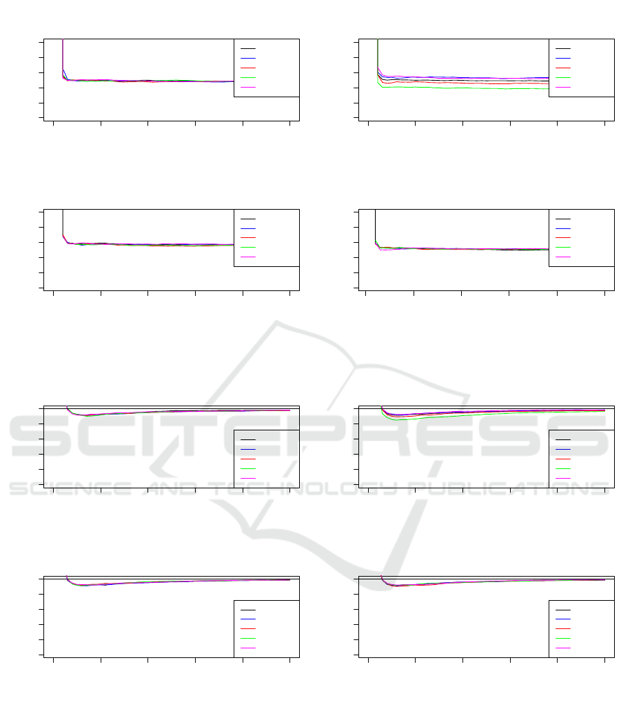
We look at the plots of the ratio ρ deﬁned by

ρ =

Variance using control variate with R

Variance using baseline with R

(35)

in Figure 1 for the Euclidean distance. ρ is a measure

of the reduction in variance using RPCV with the ma-

trix R

rather than just using R

alone. For this ratio, a

fraction less than 1 means RPCV performs better than

the baseline.

For all pairs x

except Cauchy, the reduction

of variance of the estimates of the Euclidean distance

using different R

s with RPCV converge quickly to

around the same ratio. However, when data is heavy

tailed, the choice of random projection matrix R

with

RPCV affects the reduction of variance in the esti-

mates of the Euclidean distance, and sparse matrices

have a greater variance reduction for the estimates

of the Euclidean distance.

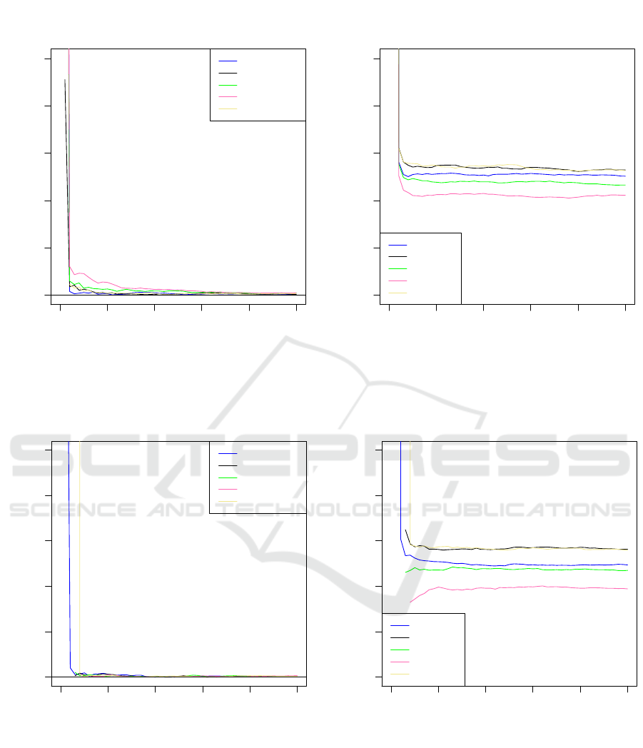
We next look at the estimates of the inner prod-

uct. In our experiments, we use Li et al., 2006a’s

method as the baseline for computing the estimates of

the inner product. Our rationale for doing this is that

both Li’s method and our method stores the marginal

norms of X, thus we should compare our method with

Li’s method for a fair comparison. The ratio of vari-

ance reduction is shown in Figure 2.

As the number of columns k of the random pro-

jection matrix R increases, the variance reduction in

our estimate of the inner product decreases, but then

increases again up to a ratio just below 1. Since Li’s

method uses an asymptotic maximum likelihood es-

timate of the inner product, then as the number of

columns of R increases, the estimate of the inner prod-

uct would be more accurate.

Thus, it is reasonable to use RPCV for Euclidean

distances, and Li’s method for inner products.

3.2 Estimating the Euclidean distance

of vectors with real data sets

We now demonstrate RPCV on two datasets, the

colon dataset from Alon et al., 1999 and the kos

dataset from Lichman, 2013.

The colon dataset is an example of a dense dataset

consisting of 62 gene expression levels with 2000 fea-

tures, and thus we have x

∈ R

2000

, 1 ≤ i ≤ 62.

The kos dataset is an example of a sparse

dataset consisting of 3430 documents and 6906 words

from the KOS blog entries, and thus we have x

∈

3430

, 1 ≤ i ≤ 6906.

We normalize each dataset such that every obser-

vation kx

= 1.

For each dataset, we consider the pairwise Eu-

clidean distances of all observations {x

}, ∀ i 6= j,

and compute the estimates of the Euclidean distance

with RPCV of the pairs {x

} which give the 20th,

30th, ..., 90th percentile of Euclidean distances.

We pick a pair in the 50th percentile for both the

colon and kos datasets (Figure 3 and Figure 4), and

show that for every different R

, the bias quickly con-

verges to zero, and that the variance reduction for the

s are around the same range. Since the bias con-

verges to zero, this implies that our control variates

work. i.e., we do not get extremely biased estimates

with lower variance.

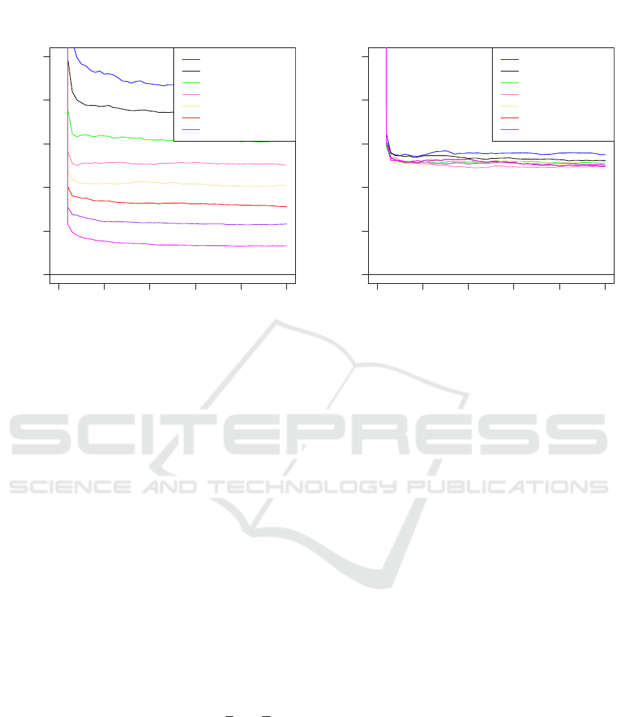
We now look at the variance reduction for pairs

from the 20th to 90th percentile of Euclidean dis-

tances from both datasets for R

(where r

i j

∼N(0,1)).

This is shown in Figure 5. We omit plots of the biases,

as well as plots of ρ varying for different random ma-

trices R

to R

since the variance reduction follows a

similar trend.

Random Projections with Control Variates

143

0 20 40 60 80 100

0.0 0.4 0.8

Plot of Ratio ρ for Pair 1 (both vectors Normal)

Number of columns k

Ratio

ρ with R1

ρ with R2

ρ with R3

ρ with R4

ρ with R5

0 20 40 60 80 100

0.0 0.4 0.8

Plot of Ratio ρ for Pair 2 (both vectors Cauchy)

Number of columns k

Ratio

ρ with R1

ρ with R2

ρ with R3

ρ with R4

ρ with R5

0 20 40 60 80 100

0.0 0.4 0.8

Plot of Ratio ρ for Pair 3 (both vectors Bernoulli)

Number of columns k

Ratio

ρ with R1

ρ with R2

ρ with R3

ρ with R4

ρ with R5

0 20 40 60 80 100

0.0 0.4 0.8

Plot of Ratio ρ for Pair 4 (IP 0)

Number of columns k

Ratio

ρ with R1

ρ with R2

ρ with R3

ρ with R4

ρ with R5

Figure 1: Plots of ρ for Euclidean Distances against number of columns in R

for each pair of vectors.

0 20 40 60 80 100

0.0 0.4 0.8

Plot of Ratio ρ for Pair 1 (both vectors Normal)

Number of columns k

Ratio

ρ with R1

ρ with R2

ρ with R3

ρ with R4

ρ with R5

0 20 40 60 80 100

0.0 0.4 0.8

Plot of Ratio ρ for Pair 2 (both vectors Cauchy)

Number of columns k

Ratio

ρ with R1

ρ with R2

ρ with R3

ρ with R4

ρ with R5

0 20 40 60 80 100

0.0 0.4 0.8

Plot of Ratio ρ for Pair 3 (both vectors Bernoulli)

Number of columns k

Ratio

ρ with R1

ρ with R2

ρ with R3

ρ with R4

ρ with R5

0 20 40 60 80 100

0.0 0.4 0.8

Plot of Ratio ρ for Pair 4 (IP 0)

Number of columns k

Ratio

ρ with R1

ρ with R2

ρ with R3

ρ with R4

ρ with R5

Figure 2: Plots of ρ for inner product against number of columns in R

for each pair of vectors.

We also see that as the Euclidean distances be-

tween vectors increases (percentile increases), we get

more variance reduction in our estimates. This in-

crease in variance reduction is strongly seen in our

dense colon dataset. Furthermore, both datasets

show substantial variance reduction regardless of the

percentile values.

4 CONCLUSION AND FUTURE

WORK

We have presented a new method RPCV which works

well in conjunction with different random projection

matrices to reduce the variance of the estimates of

the Euclidean distance and inner products on differ-

ICPRAM 2017 - 6th International Conference on Pattern Recognition Applications and Methods

144

0 20 40 60 80 100

0.00 0.02 0.04 0.06 0.08 0.10

Bias using Control Variates (Colon)

Number of columns k

Bias

Bias with R1

Bias with R2

Bias with R3

Bias with R4

Bias with R5

0 20 40 60 80 100

0.0 0.2 0.4 0.6 0.8 1.0

Plot of ρ (Colon)

Number of columns k

Ratio

ρ with R1

ρ with R2

ρ with R3

ρ with R4

ρ with R5

Figure 3: Plots of bias and variance reduction of Euclidean distances at 50th percentile against number of columns in R

for

colon data.

0 20 40 60 80 100

0.00 0.02 0.04 0.06 0.08 0.10

Bias using Control Variates (Kos)

Number of columns k

Bias

Bias with R1

Bias with R2

Bias with R3

Bias with R4

Bias with R5

0 20 40 60 80 100

0.0 0.2 0.4 0.6 0.8 1.0

Plot of ρ (Kos)

Number of columns k

Ratio

ρ with R1

ρ with R2

ρ with R3

ρ with R4

ρ with R5

Figure 4: Plots of bias and variance reduction of Euclidean distances at 50th percentile against number of columns in R

for

kos data.

ent types of vectors x

, x

. This allows for more accu-

rate estimates of the Euclidean distance. As the Eu-

clidean distance between two vectors increases, we

expect greater variance reduction. In essence, we

have shown that it is possible to juxtapose statistical

variance reduction methods with random projections

to give better results.

While RPCV gives a variance reduction for the es-

timates of the inner products, the ratio of variance re-

duction becomes minimal as the number of columns

increases when compared to Li’s method. This is not

surprising since Li’s method for estimating the inner

products is an asymptotic maximum likelihood esti-

mator, and is extremely accurate as the number of

Random Projections with Control Variates

145

0 20 40 60 80 100

0.0 0.2 0.4 0.6 0.8 1.0

Plot of ρ for percentiles with R_1 (Colon)

Number of columns k

Ratio

ρ at 20th percentile

ρ at 30th percentile

ρ at 40th percentile

ρ at 50th percentile

ρ at 60th percentile

ρ at 70th percentile

ρ at 80th percentile

0 20 40 60 80 100

0.0 0.2 0.4 0.6 0.8 1.0

Plot of ρ for percentiles with R_1 (Kos)

Number of columns k

Ratio

ρ at 20th percentile

ρ at 30th percentile

ρ at 40th percentile

ρ at 50th percentile

ρ at 60th percentile

ρ at 70th percentile

ρ at 80th percentile

Figure 5: Plots of ρ for percentiles of Euclidean distance for R

in both colon and kos data.

columns increases.

Although RPCV requires storing marginal norms

and computing the covariance between two p dimen-

sional vectors, the cost of doing so is negligible when

compared to matrix multiplication. Furthermore, the

computation of marginal norms is unnecessary when

the data is already normalized.

In fact, RPCV can be seen as a method that nicely

complements Li’s method since both methods require

storing marginal norms. RPCV substantially reduces

the errors of the estimates of the Euclidean distance,

while Li’s method substantially reduces the errors of

the estimates of the inner product.

We note that different applications may require a

certain type of random projection matrix. Thus if we

want to reduce the errors in our estimates, we can-

not just switch to a different random projection matrix

where the entries allow us to place sharper probability

bounds on our errors. If we want data to be invari-

ant under rotations, then a Normal random projection

matrix would be best suited (Mardia et al., 1979). If

we wanted to desparsify data, then a random projec-

tion matrix with i.i.d. entries from {−

√

p,0,

√

p}, p

small might be preferred (Achlioptas, 2003). If we

are focused on speed and quick information retrieval,

then very sparse random projections (Li et al., 2006b)

or random projection matrices formed by the SHRT

(Boutsidis and Gittens, 2012) would be more prefer-

able. RPCV allows us to reduce the error in all these

estimates.

While we have demonstrated good empirical re-

sults in the variance reduction for Euclidean distances

for RPCV, we still need an expression for the ﬁrst and

second moments of A + c(B −µ

) when the elements

in the random projection matrix R are correlated in

order to theoretically show that RPCV does achieve

this reduction in variance. We are currently working

on this.

Finally, we want look forward to extending this

method of control variates to other applications of

random projections.

REFERENCES

Achlioptas, D. (2003). Database-friendly Random Projec-

tions: Johnson-Lindenstrauss with Binary Coins. J.

Comput. Syst. Sci., 66(4):671–687.

Ailon, N. and Chazelle, B. (2009). The Fast Johnson-

Lindenstrauss Transform and Approximate Nearest

Neighbors. SIAM J. Comput., 39(1):302–322.

Alon, U., Barkai, N., Notterman, D., Gish, K., Ybarra, S.,

Mack, D., and Levine, A. (1999). Broad patterns

of gene expression revealed by clustering analysis of

tumor and normal colon tissues probed by oligonu-

cleotide arrays. Proceedings of the National Academy

of Sciences, 96(12):6745–6750.

Boutsidis, C. and Gittens, A. (2012). Improved matrix al-

gorithms via the subsampled randomized hadamard

transform. CoRR, abs/1204.0062.

Boutsidis, C., Zouzias, A., and Drineas, P. (2010). Random

projections for k-means clustering. In Lafferty, J. D.,

Williams, C. K. I., Shawe-Taylor, J., Zemel, R. S., and

Culotta, A., editors, Advances in Neural Information

ICPRAM 2017 - 6th International Conference on Pattern Recognition Applications and Methods

146

Processing Systems 23, pages 298–306. Curran Asso-

ciates, Inc.

Fern, X. Z. and Brodley, C. E. (2003). Random projection

for high dimensional data clustering: A cluster ensem-

ble approach. pages 186–193.

Li, P. and Church, K. W. (2007). A Sketch Algorithm for

Estimating Two-Way and Multi-Way Associations.

Comput. Linguist., 33(3):305–354.

Li, P., Hastie, T., and Church, K. W. (2006a). Improving

Random Projections Using Marginal Information. In

Lugosi, G. and Simon, H.-U., editors, COLT, volume

4005 of Lecture Notes in Computer Science, pages

635–649. Springer.

Li, P., Hastie, T. J., and Church, K. W. (2006b). Very Sparse

Random Projections. In Proceedings of the 12th

ACM SIGKDD International Conference on Knowl-

edge Discovery and Data Mining, KDD ’06, pages

287–296, New York, NY, USA. ACM.

Liberty, E., Ailon, N., and Singer, A. (2008). Dense fast ran-

dom projections and lean walsh transforms. In Goel,

A., Jansen, K., Rolim, J. D. P., and Rubinfeld, R.,

editors, APPROX-RANDOM, volume 5171 of Lecture

Notes in Computer Science, pages 512–522. Springer.

Lichman, M. (2013). UCI machine learning repository.

Mardia, K. V., Kent, J. T., and Bibby, J. M. (1979). Multi-

variate Analysis. Academic Press.

Paul, S., Boutsidis, C., Magdon-Ismail, M., and Drineas, P.

(2012). Random Projections for Support Vector Ma-

chines. CoRR, abs/1211.6085.

Ross, S. M. (2006). Simulation, Fourth Edition. Academic

Press, Inc., Orlando, FL, USA.

Vempala, S. S. (2004). The Random Projection Method,

volume 65 of DIMACS series in discrete mathematics

and theoretical computer science. Providence, R.I.

American Mathematical Society. Appendice p.101-

105.

APPENDIX

While computing ﬁrst and second moments neces-

sarily require lots of algebra, we use the following

lemma for ease of computation.

Lemma 4.1. Suppose we have a sequence of terms

}

i=1

= {a

}

i=1

for a = (a

,...,a

), {s

}

i=1

}

i=1

for b = (b

,...,b

) and r

i.i.d. random

variables with E[r

] = 0, E[r

] = 1 and ﬁnite third, and

fourth moments, denoted by µ

,µ

respectively.

Then:





∑

i=1





∑

i=1

= kak

(36)





∑

i=1





= µ

∑

i=1

+ 6

p−1

∑

u=1

∑

v=u+1

(37)

∑

i=1

∑

i=1

∑

i=1

= ha, bi (38)





∑

i=1

∑

i=1





∑

i=1

∑

i6= j

+ 4

p−1

∑

u=1

∑

v=u+1

(39)

The motivation for this lemma is that we do ex-

pansion of terms of the above four forms to prove our

theorems.

Random Projections with Control Variates

147