Reactive Agent-based Model for Convergence of Autonomous Vehicles to

Parallel Formations Heading to Predeﬁned Directions of Motion

Vander L. S. Freitas

and Elbert E. N. Macau

National Institute for Space Research - INPE, 12227-010, S

ao Jos

e dos Campos, Brazil

Laboratory of Computing and Applied Mathematics, National Institute for Space Research - INPE, 12227-010,

ao Jos

e dos Campos, Brazil

Keywords:

Reactive Agents, Parallel Formation, Collective Motion.

Abstract:

In this work we introduce a reactive agent-based model for convergence of autonomous vehicles to parallel

formations heading to predeﬁned directions of motion. They interact via rules of repulsion, alignment and

attraction. There is also an abstraction of the desired path of motion, represented by a virtual guiding vehicle,

which shows the desired direction to be followed by the formation. We performed simulations with different

combinations of interaction rules and studied the parameter space. Additionally, we simulate the occurrence

of communication failure among agents and the presence of noise. The resulting formations are evaluated by

three quantiﬁers.

1 INTRODUCTION

Nature exhibits many emergent motions in collections

of living beings. These emergent order behaviors

are the result of local interactions among the agents.

Common situations of the emergence of collective

motion are in predator escaping, food search or hunt-

ing, for example.

Collective motion is a phenomenon that occurs

in collections of agents, similar or not, who interact

with each other, resulting in ordered motion (Vicsek

and Zafeiris, 2012). Those interactions can be among

close neighbors or in the context of a more evolved

framework. Collective motion is present everywhere,

from colonies of bacteria to schools of ﬁsh (Paley

et al., 2007). There are about 1 million species of

known insects in the world (Chapman et al., 2009)

and despite most of them live lonely, many others are

famous because of their organized behavior (Vicsek

and Zafeiris, 2012).

The motivation for the study of collective motion

is to understand the interaction rules among the units.

These rules may be applied to artiﬁcial vehicles so

they can work collaboratively in some tasks. Then it

is possible to establish a link between control theory

and applications of collective like robot swarms.

Studies on collective motion have resulted on

models that attempt to recreate the observed collec-

tive arrangements of agents (Reynolds, 1987; Vicsek

et al., 1995; Czir

ok et al., 1999; Couzin et al., 2002;

Paley, 2007; Cucker and Smale, 2007; Veerman et al.,

2005; Dafﬂon et al., 2013). They are used in many

applications like satellites in ﬂight formation (Salazar,

2012), unmanned aerial vehicles (Klein, 2005) (Park

et al., 2015), unmanned subaquatic vehicles (Leonard

et al., 2007), aquatic surface robots (Duarte et al.,

2016) and others.

In this work we propose a reactive agent-based

model for convergence of autonomous vehicles to

moving formations. The aim is to group the vehi-

cles inside a moving bounded area heading to a prede-

ﬁned direction. The agents interact via rules of repul-

sion, alignment and attraction, similar to the works

of Reynolds (Reynolds, 1987). The main difference

is that here there is an individual called virtual agent

(VA), i.e., a “virtual vehicle” that represents the de-

sired path we want to be followed by the formation.

It is not a real vehicle of the model but an abstrac-

tion. The individuals begin at random positions inside

an area and after a transient of interactions they con-

verge to a moving formation that heads in parallel to

the same direction of motion of the VA.

The behavior of the virtual agent is similar to a

leader, or the stakeholder agents of (Kerman et al.,

2012), which have privileged information about the

desired direction of the motion. The main difference

is that, as mentioned before, it is not a real vehicle but

an abstraction.

166

L. S. Freitas V. and E. N. Macau E.

Reactive Agent-based Model for Convergence of Autonomous Vehicles to Parallel Formations Heading to Predeﬁned Directions of Motion.

DOI: 10.5220/0006187201660173

In Proceedings of the 9th International Conference on Agents and Artiﬁcial Intelligence (ICAART 2017), pages 166-173

ISBN: 978-989-758-219-6

One possible usage of the VA would be to consider

it as a moving GPS signal. In this case, one should

expect the agents to converge in a parallel formation

around its signal coordinates. Considering a scenario

in which the vehicles are disperse in an environment

and doing some work, e.g., measuring temperature, if

one wants them to head to another geographic loca-

tion, our model would be a good choice since VA dic-

tates the path for the ﬂock. Additionally, the model

has the advantage of making the individuals getting

together, which is useful to group disperse agents.

(Duarte et al., 2016) presented controls using neu-

ral networks and one of the tasks their aquatic robots

can do is to go towards a geographic location. The

role of our virtual agent is also to point out coordi-

nates to be followed, but with the difference that these

coordinates change through time.

The interaction rules have biological inspiration,

derived from ﬁshes and birds. (Herbert-Read et al.,

2011) analyzed 2D trajectories of birds and observed

rules of attraction and repulsion between close neigh-

bors. In a similar work, (Katz et al., 2011) found out

that ﬁshes change their trajectories depending on the

neighbors in front of them. In this work we present

strategies for attraction and repulsion usage in the

context of ordered motion.

We performed experiments in parameter space to

seek for formations according to speciﬁc objectives.

Besides, we simulated communication problems, by

adding a probability distribution of individuals not re-

sponding to the environment stimuli on each time in-

stant. Lastly, we veriﬁed the model behavior in the

presence of a random noise. Both noise and com-

munication failures have to be considered when de-

signing real systems of this kind (Duarte et al., 2016),

because the individuals have sensors with limited pre-

cision. Also, there are environmental issues like the

presence of wind, for aquatic robots, or terrain irreg-

ularities for terrestrial vehicles, etc.

The paper is organized as follows. Section 2 de-

tails the reactive model, Section 3 presents implemen-

tation details, Section 4 reports some simulation re-

sults and Section 5 shows our conclusions.

2 REACTIVE MODEL

This model is called reactive because it uses the ar-

chitecture of reactive agents, in which the individuals

do not keep information of the past, but only respond

to the current state of the system (Russell and Norvig,

2003).

The components of our proposed model are the

so-called virtual agent, with its interaction radius, and

Figure 1: Model components: Virtual agent is in blue,

agents are in red and VAIR is in green.

the reactive agents, as follows (Figure 1):

• Virtual Agent: Its role is to point out the desired

motion direction and the moving region in which

we want that the agents to form a parallel forma-

tion. Despite its interaction with agents, it is not a

real agent but an abstraction.

• Virtual Agent Interaction Radius (VAIR): Cir-

cular region centered in VA, inside which the par-

allel formation will converge.

• Reactive Agents: The agents of the model. They

model autonomous vehicles. Their main charac-

teristic is that they do not keep memory of previ-

ous interactions, i.e., they respond to the current

system state according to simple rules.

The aim here is to make the agents to enter the

VAIR and follow the VA in a parallel formation. For

this purpose they interact via adjustments in their ve-

locity module (speed) and rules (interaction strengths)

based on repulsion, alignment and attraction. We call

these interaction rules as “virtual forces”. Here the

concept of force is related to how the presence of the

neighbors of an agent i can impose changes on its

heading angle θ

= θ

(t).

The speed adjustment is performed according to

the position of the agent in relation to the VAIR.

When an agent is outside the VAIR its speed is higher

than when it is inside, because it needs to reach the

VA. When an agent is entering the VAIR it suffers a

deceleration according to Eq 1, so it can move along

with the VA. The idea is to guarantee that the parallel

formation will occur inside the VAIR.

| = |v

| −

(|v

ini

| − |v

|)(t −t

)

∆t

(1)

so that v

is the velocity of agent i, v

is the velocity

of the VA, v

ini

is the velocity of agent i at the moment

it started entering the VAIR, t is the current time, t

the time instant in which the acceleration will ﬁnish

and ∆t

is the total time of this procedure.

In this equation ∆t

= t +rnd, in which t represents

the approximate time for the agent to move from the

Reactive Agent-based Model for Convergence of Autonomous Vehicles to Parallel Formations Heading to Predeﬁned Directions of Motion

167

VAIR boundary to the VA’s position, and rnd is a ran-

dom number in the interval rnd ∈ (−γ, γ). Here we

used γ

= t to guarantee a homogeneous distribution

of agents inside the VAIR.

When an agent is leaving the VAIR, its speed in-

creases according to Eq 2. In this case, |v

out

| repre-

sents the maximum speed outside the VAIR.

| = |v

| −

(|v

out

| − |v

ini

|)(t −t

)

∆t

(2)

We use ﬁve interaction rules to achieve the paral-

lel formation in the desired direction of motion. The

rules are written in the form of imposed control ac-

tions, or “forces”, as follows (Figure 2):

• F

(Alignment): Orders the agent to align with the

average heading angles of its neighbors.

• F

(Cohesion): Orders the agent to go to the center

of mass of its neighbors.

• F

(Alignment with virtual agent): Orders the

agent to align with the VA heading angle.

• F

(Cohesion with virtual agent): Orders the

agent to move towards the VA.

• F

(Separation): Orders the agent to move apart

from its nearest neighbor.

All of those control actions are applied to the

agent as the angular velocity control input, acting di-

rectly on the heading angle of the agents at discrete

time. Their maximum value is 1.00 decimal degree

per time unit to account for limitations that may be

present in the heading angle changes of real robots.

For example, if agent 1 has θ

= 150.00 as its head-

ing angle, and VA θ

= 160.00, when F

is applied

it will result in F

= 1.00 and θ

= 151.00. How-

ever, if θ

= 159.50 and θ

= 160.00 and F

is ap-

plied, the result would be F

= 0.50 and consequently

= 160.00. Each time unit (tu) corresponds to a

travel of 1.00 bl (body length of an agent) of VA, i.e.,

the VA’s speed is |v

| = 1 bl/tu.

and F

do the same than alignment and co-

hesion rules deﬁned by Reynolds (Reynolds, 1987).

Each isolated force produces an effect but we are in-

terested on the combinations of them. For this case

the resulting force F is calculated as a linear combi-

nation of the ﬁve forces, according to Eq 3.

F(t) =

(t) + α

(t)

+ α

(3)

in which α

, α

are control coefﬁcients and

each force is unitary. The separation force does not

appear here because it is used isolated when a colli-

sion between two individuals is about to happen. In

this case, we use Eq 4.

(a) F

(b) F

(d) F

(e) F

Figure 2: Interaction rules. The dotted circumferences rep-

resent the interaction area (vision radius) of one agent (in

black). At (d) and (e) the blue agent is the virtual agent.

F(t) = F

(t) (4)

The dynamics of an agent is given by Eq 5.

˙x

= |v

|. cos(θ

)

˙y

= |v

|. sin(θ

)

= F

(5)

where [x

, y

]

∈ R

is the ith agent’s position, ex-

pressed in terms of polar coordinates.

The virtual agent represents the desired trajectory

for the parallel formation, i.e., the position over time

that we want our formation to follow. Its dynamics

works as an ordinary agent but with ﬁxed heading an-

gle θ

, velocity |v

| = |v

3 IMPLEMENTATION

The simulations were implemented using the Python

language and some libraries like matplotlib

and

numpy

, for ploting, random number generation, etc.

The simulation scenario works as a torus. When

the agents reach the outskirts of the environment, they

appear at the opposite side, heading to the same direc-

tion as before. For example, when they are heading to

the left and cross the limits they appear at right.

Agents begin in a bounded rectangular area be-

hind the VA, with random coordinates and heading

angles as shown in Figure 1. The coordinate system

is given by the size of the agent. We assumed that the

VA is able to move the distance of one body length

(bl) per time unit (tu). Considering that particles have

a circular shape, this bl is their diameter.

The implementation has basically three classes:

Agent, Model and Simulation. Agent represents each

http://matplotlib.org/

http://www.numpy.org/

ICAART 2017 - 9th International Conference on Agents and Artiﬁcial Intelligence

168

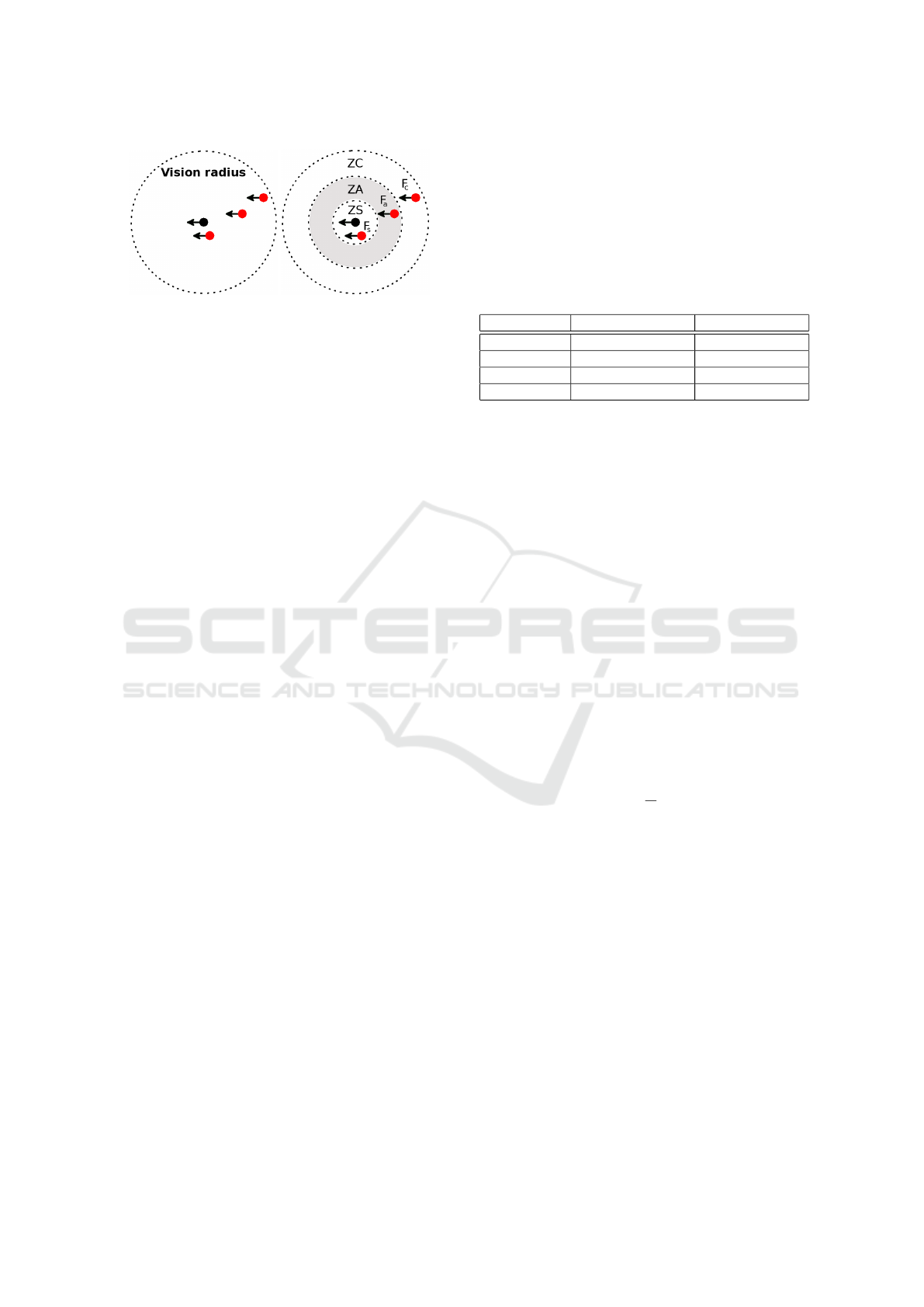
(a) C-1 (b) C-2

Figure 3: Calculation of forces: S-1) Considering the entire

agent vision radius equally; and S-2) Considering zones of

perception (ZS - Zone of separation, ZA - Zone of align-

ment and ZC - Zone of cohesion). The black agent is an

ordinary agent of the model and the dotted region corre-

sponds to its vision region (perception region). Agents in

red are its neighbors.

agent of the simulation, with its coordinates and

speed. When the agent enters or leaves the VAIR, its

speed changes through Eqs. 1 and 2. The class Model

has a list of agents and is responsible for evolving the

model, according to the Eq. 5, parameters like neigh-

borhood radius, control coefﬁcients α

, α

and the chosen strategy. The strategies are presented

in the next section. The class Simulation is respon-

sible for setting up the parameters of the model and

running the simulations.

4 RESULTS

There are two approaches to deal with the neighbor-

hood of each agent. In the ﬁrst (S-1) the agent consid-

ers a neighborhood radius in which every neighbor is

treated similarly, i.e., the control actions (forces) are

applied without distinction, regarding their position

(Figure 3a).

The second approach (S-2) takes into account the

distances between the agent and its neighbors through

perception zones (Figure 3b). In this case, when a

neighbor is in the ﬁrst radius, closer to the agent, only

is calculated. Following the same logic, when the

neighbor is in the second zone (ZA), only the force of

alignment F

is computed, and in the third zone (ZC),

only F

is considered. This approach is inspired in

an observed behavior that occurs in schools of ﬁsh.

(Katz et al., 2011) showed that some species of ﬁsh

increase their speed when a neighbor is far ahead (at-

traction), while decreases when it is too close (sepa-

ration). (Kerman et al., 2012) has implemented these

three perception zones but the outer region (ZC) con-

tains the other two inside, and ZA contains ZS. Here

we consider them as rings, i.e., they do not overlap,

similar to the works of (Couzin et al., 2002).

We test four strategies (combinations of forces) as

shown in Table 1. The application of forces depends

on whether the agent is inside or outside the VAIR.

Despite there are only four strategies, the table shows

eight possibilities because of the two approaches of

neighborhood calculation, S-1 and S-2.

Table 1: Strategies (combinations of control actions) used

when the agents are inside or outside the VAIR.

Strategy

Outside the VAIR Inside the VAIR

S-1.1 (S-2.1)

, F

S-1.2 (S-2.2) F

, F

S-1.3 (S-2.3)

, F

S-1.4 (S-2.4)

, F

Deﬁnition 1 If all agents are moving in a parallel

formation inside the VAIR and have the same speed of

the virtual agent, then they are in a Desired Formation

(DF).

We consider they are in parallel if the higher dif-

ference between the VA heading angle θ

and each

agent heading angle θ

is smaller than an imposed tol-

erance β

lim

. In other words, they are in parallel if

|θ

− θ

| < β

lim

, for i ∈ {1, 2, · · · ,N}.

We deﬁne three quantiﬁers to measure what kind

of parallel formations we can get with different com-

binations of control actions:

1. Temporal index (τ): time units (tu) from the be-

ginning of the simulation until the DF.

2. Angular uniformity index (φ): The relative angles

between the position of each agent and the VA

is calculated. Then the order parameter (Eq 6 -

(Strogatz, 2000)) is evaluated with those angles.

∑

j=1

iΘ

(6)

with e

iΘ

= cos Θ

+ i sin Θ

In this case, φ = |p

|. When φ = 0 the agents

are uniformly distributed around the VA. On the

other hand, if φ = 1 then the agents are at the same

position.

3. Radial uniformity index (ρ): The mean of the dis-

tances between each agent and the VA.

The ﬁrst index (τ) computes the total time for the

model convergence, and the two others, φ and ρ, are

related to the distribution of the formation. If the

agents are very close to each other, they have small ρ.

For the case in which the agents converge to straight

lines, following the VA, φ is near 1. On the other

hand, when the agents converge to some sort of cir-

cular shape, centered in VA, φ is close to zero.

Reactive Agent-based Model for Convergence of Autonomous Vehicles to Parallel Formations Heading to Predeﬁned Directions of Motion

169

We evaluated the strategies with all combinations

of α

, α

∈ {1, 2, ··· , 10}. Each conﬁgura-

tion is simulated 10 times using random initial posi-

tions and heading angles θ

θ = (θ

(t))

i=1,2,···,N

Initial conditions:

• Population of N = 12 agents randomly positioned

inside a rectangle of dimensions 36 x 76 bl, as

shown in Figure 1.

• Vision radius of each agent: 5.5 bl.

• Minimum separation: 2.5 bl.

• F

: 2 decimal degrees.

• F

= F

: 1 decimal degree.

• Heading angles θ

θ: Random.

• |v

| = 1 bl/tu , |v

out

| = 1.4 bl/tu.

• VAIR: 25 bl.

• Virtual agent heading angle: 180 decimal degrees.

• β

lim

: 5 decimal degrees.

Only cases that reach the DF for all 10 attempts

and obeying τ ≤ 3000 tu are considered. Simulations

are limited to this temporal limit of 3000 tu due to

the large number of combinations in parameter space.

Also, this value is set because the agents usually con-

verge in less than 2000 tu, according to experimental

observations.

We calculate the three indexes for each combina-

tion of control coefﬁcients. Figure 4 depicts the de-

sired formations achieved in terms of the maximum

and minimum values of τ, φ and ρ.

(a) min(τ) =

871: S-2.2

(b) max(τ) =

1971: S-1.1

0.09: S-1.3

(d) max(φ) =

0.36: S-1.4

(e) min(ρ) =

5.20: S-1.2

(f) max(ρ) =

13.88: S-2.4

Figure 4: Desired formations for the simulated conﬁg-

urations in terms of the maximum and minimum values

achieved for τ, φ and ρ. Conﬁgurations: (a) S-2.2: α

= 8,

= 9 and α

= 4; (b) S-1.1: α

= 7, α

= 1 and α

= 3;

= 1, α

= 4, α

= 4 and α

= 9; (d) S-1.4:

= 3, α

= 5, α

= 7 and α

= 9; (e) S-1.2: α

= 3,

= 10 and α

= 10; (f) S-2.4: α

= 2, α

= 3, α

= 6

and α

= 9.

If one wants agents to converge as fast as possi-

ble, a good choice would be strategy S-2.2 with the

conﬁguration of Figure 4a. An example of simulation

with this conﬁguration is shown in Figure 5. Other-

wise, if the aim is to get them very close to each other

the best option is the conﬁguration of strategy S-1.2 of

Figure 4e. The resulting formations depends on both

the chosen strategy and conﬁguration. In this sense,

some strategies are more suitable for some objectives

than others.

In a situation in which one desires the agents to

spread uniformly inside the VAIR, φ would be near

zero and ρ around the half of VAIR size. Consider-

ing an application in which surveillance vehicles are

monitoring an area it is expected that they travel far

from each other, so they can explore a bigger area.

For this purpose, ρ should be as large as possible.

Certain combinations of parameters α do not lead

to the expected convergence. If one sets the α

value

much higher than α

, it is possible that the agents

never follow the VA because they are more likelly to

converge to a parallel motion heading elsewere. Fig-

ure 6 shows the dependence between α

and α

for

strategy S-2.2, in which the colors correspond to the

rate of DF convergence. The agents are more likely to

reach the DF when α

≥ α

, for S-2.2.

We simulate failures on communication, emulat-

ing what would happen case an agent lost the feed-

back from its neighbors during a time unit. In our

setup, this problem does not last until the end of the

simulation, but it is calculated each time unit. Also,

we add a random noise to the dynamics of their head-

ing angles, to simulate external interferences from the

environment (wind, terrain irregularities, etc) and sen-

sor imprecisions.

The random noise ε ∈ [−δ, δ] is applied according

to Eq. 7, with δ representing the noise strength. There

is also a probability p of the agent to ignore its neigh-

bors stimuli. We simulate both noise and communica-

tion failure for each agent, independently, to account

for what would happen in a real world system.

θ = F + ε (7)

We have chosen strategy S-2.2 with the conﬁgu-

ration of Figure 4a to simulate noise and communi-

cation failures, because it converges faster than the

others.

We varied p ∈ [0, 0.9] and δ ∈ [0, 0.9], with steps

of ∆p = ∆δ = 0.1, and calculated the average of 50

simulations for each pair (p, δ) since initial conditions

are random. Figure 7a shows the results. Seems like

for p ∈ [0, 0.8] there is no change in the colors, be-

cause of the abrupt difference between p = 0.8 and

p = 0.9. Figure 7b presents this region in more de-

ICAART 2017 - 9th International Conference on Agents and Artiﬁcial Intelligence

170

(a) t = 2 tu

(b) t = 383 tu

(d) t = 870 tu

Figure 5: Simulation of strategy S-2.2 with conﬁguration

= 8, α

= 9 and α

= 4.

tails. As expected, the higher the value of p the longer

it takes to reach the desired formation, with τ increas-

ing smoothly for p ∈ [0, 0.8]. When p = 0.9 it sud-

denly jumps to a very high value. It probably hap-

pened because for S-2.2 the only force acting outside

the VAIR is F

. If the agents ignore it with a proba-

bility of p = 0.9, than they will only try to go towards

Figure 6: Convergence ratio when varying control coefﬁ-

cients α

and α

for strategy S-2.2. Colors represent the

convergence ratio and white regions represent the cases in

which DF was not achieved. The agents are more likely to

reach the DF when α

≥ α

VA 10% of the cases, resulting in a very high τ.

The values of ε were proportional to

θ and it seems

like ε does not affect the convergence of formations,

according to Figure 7.

Results have shown that this model is quite re-

silient to communication failures, and the presence

of noise, since their impact was small, specially for

noise.

5 CONCLUSIONS

We presented a reactive agent-based model whose

aim is to make agents converge to parallel formations

heading to a desired direction. We introduced the so-

called virtual agent, whose role is to indicate the for-

mations direction of motion and also to evaluate their

shapes. The agents interact via ﬁve rules depending

on a chosen strategy (combination of rules) and a con-

ﬁguration (weight of each rule).

Four strategies were evaluated and analyzed for

about 44,000 conﬁgurations, considering two neigh-

borhood approaches to calculate the virtual forces:

one taking into account the presence of neighbors

likewise, and the other using non-overlapping inter-

action zones.

The last simulations were focused on communi-

cation failures, in which the agents had a probability

of ignoring the external stimuli from neighbors, each

time unit. This represents failures on the wireless net-

work, or even the GPS signal. Besides, we added a

random additive noise to the agents heading angle, to

account for the sensors imprecision, and environmen-

Reactive Agent-based Model for Convergence of Autonomous Vehicles to Parallel Formations Heading to Predeﬁned Directions of Motion

171

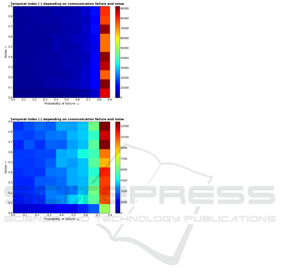
(a)

(b)

Figure 7: Temporal index (τ) depending on the probability

of communication failure p and a random noise ε ∈ [−δ, δ],

for S-2.2, with α

= 8, α

= 9 and α

= 4. (a) communi-

cation failure with p ∈ [0, 0.9], (b) Zooming to p ∈ [0, 0.8].

Color represents τ.

tal issues as the presence of wind or terrain irregu-

larities. Results have shown that our model is quite

resilient to communication failures, and the presence

of noise, since their impact was small, specially for

noise.

Considering that agents have sensory limitations,

one can use this model as a pre-step before switching

to another model with more controls, since its princi-

ple is to group agents into a bounded region.

ACKNOWLEDGEMENTS

The authors would like to thank the Conselho Na-

cional de Desenvolvimento Cientiﬁco e Tecnologico

- CNPq, and the Coordenacao de Aperfeicoamento

de Pessoal de Nivel Superior - CAPES, for the ﬁ-

nancial support. EENM thanks FAPESP, processes

2011/50151-0 and 2015/50122-0, and CNPq, process

458070/2014-9, for their support.

REFERENCES

Chapman, A. D., Study., A. B. R., and Australia. (2009).

Numbers of living species in Australia and the world /

Arthur D. Chapman. Department of the Environment,

Water, Heritage and the Arts [Canberra, ACT].

Couzin, I. D., Krause, J., James, R., Ruxton, G. D., and

Franks, N. R. (2002). Collective memory and spatial

sorting in animal groups. Journal of Theoretical Biol-

ogy, 218(1):1 – 11.

Cucker, F. and Smale, S. (2007). Emergent behavior in

ﬂocks. IEEE Transactions on Automatic Control,

pages 852–862.

Czir

ok, A., Barab

asi, A.-L., and Vicsek, T. (1999). Collec-

tive motion of self-propelled particles: Kinetic phase

transition in one dimension. Phys. Rev. Lett., 82:209–

212.

Dafﬂon, B., Gechter, F., Gruer, P., and Koukam, A. (2013).

Vehicle platoon and obstacle avoidance: A reactive

agent approach. IET Intelligent Transport Systems,

7(3):257–264.

Duarte, M., Costa, V., Gomes, J., Rodrigues, T., Silva, F.,

Oliveira, S. M., and Christensen, A. L. (2016). Evolu-

tion of collective behaviors for a real swarm of aquatic

surface robots. PLOS ONE, 11(3):1–25.

Herbert-Read, J. E., Perna, A., Mann, R. P., Schaerf, T. M.,

Sumpter, D. J. T., and Ward, A. J. W. (2011). Inferring

the rules of interaction of shoaling ﬁsh. Proceedings

of the National Academy of Sciences, 108(46):18726–

18731.

Katz, Y., Tunstrom, K., Ioannou, C. C., Huepe, C., and

Couzin, I. D. (2011). Inferring the structure and dy-

namics of interactions in schooling ﬁsh. Proceedings

of the National Academy of Sciences, 108(46):18720–

18725.

Kerman, S., Brown, D., and Goodrich, M. A. (2012). Sup-

porting human interaction with robust robot swarms.

In Resilient Control Systems (ISRCS), 2012 5th Inter-

national Symposium on, pages 197–202.

Klein, J. K. (2005). Controlled Collective Motion for Mul-

tivehicle Trajectory Tracking. Master’s thesis, Univer-

sity of Washington, USA.

Leonard, N., Paley, D., Lekien, F., Sepulchre, R., Fratan-

toni, D., and Davis, R. (2007). Collective motion, sen-

sor networks, and ocean sampling. Proceedings of the

IEEE, 95(1):48–74.

Paley, D., Leonard, N. E., Sepulchre, R., Gr

unbaum, D.,

and Parrish, J. K. (2007). Oscillator models and col-

lective motion: Spatial patterns in the dynamics of en-

gineered and biological networks. IEEE Control Sys-

tems Magazine, 27(4):89–105.

Paley, D. A. (2007). Cooperative control of collective mo-

tion for ocean sampling with autonomous vehicles.

PhD thesis, Princeton University.

ICAART 2017 - 9th International Conference on Agents and Artiﬁcial Intelligence

172

Park, C., Cho, N., Lee, K., and Kim, Y. (2015). Formation

ﬂight of multiple uavs via onboard sensor information

sharing. Sensors, 15:17397–17419.

Reynolds, C. W. (1987). Flocks, herds and schools: A

distributed behavioral model. SIGGRAPH Comput.

Graph., 21(4):25–34.

Russell, S. J. and Norvig, P. (2003). Artiﬁcial Intelligence.

Pearson Education, 2 edition.

Salazar, F. J. T. (2012). Deployment and maintenance of a

satellite formation ﬂight around L4 and L5 lagrangian

points in the earth-moon system based on low cost

strategies. PhD thesis, Instituto Nacional de Pesquisas

Espaciais.

Strogatz, S. H. (2000). From kuramoto to crawford: Ex-

ploring the onset of synchronization in populations of

coupled oscillators. Phys. D, 143(1-4):1–20.

Veerman, J. J. P., Lafferriere, G., Caughman, J. S., and

Williams, A. (2005). Flocks and formations. Journal

of Statistical Physics, 121(5):901–936.

Vicsek, T., Czir

ok, A., Ben-Jacob, E., Cohen, I., and

Shochet, O. (1995). Novel type of phase transition

in a system of self-driven particles. Phys. Rev. Lett.,

75:1226–1229.

Vicsek, T. and Zafeiris, A. (2012). Collective motion.

Physics Reports, 517(3-4):71 – 140. Collective mo-

tion.

Reactive Agent-based Model for Convergence of Autonomous Vehicles to Parallel Formations Heading to Predeﬁned Directions of Motion

173