The Possibilistic Reward Method and a Dynamic Extension for the

Multi-armed Bandit Problem: A Numerical Study

Miguel Mart

ın, Antonio Jim

enez-Mart

ın and Alfonso Mateos

Decision Analysis and Statistics Group, Universidad Polit

ecnica de Madrid,

Campus de Montegancedo S/N, Boadilla del Monte, Spain

Keywords:

Multi-armed Bandit Problem, Possibilistic Reward, Numerical Study.

Abstract:

Different allocation strategies can be found in the literature to deal with the multi-armed bandit problem under

a frequentist view or from a Bayesian perspective. In this paper, we propose a novel allocation strategy, the

possibilistic reward method. First, possibilistic reward distributions are used to model the uncertainty about

the arm expected rewards, which are then converted into probability distributions using a pignistic probability

transformation. Finally, a simulation experiment is carried out to ﬁnd out the one with the highest expected

reward, which is then pulled. A parametric probability transformation of the proposed is then introduced

together with a dynamic optimization, which implies that neither previous knowledge nor a simulation of the

arm distributions is required. A numerical study proves that the proposed method outperforms other policies

in the literature in ﬁve scenarios: a Bernoulli distribution with very low success probabilities, with success

probabilities close to 0.5 and with success probabilities close to 0.5 and Gaussian rewards; and truncated in

[0,10] Poisson and exponential distributions.

1 INTRODUCTION

The multi-armed bandit problem has been at great

depth studied in statistics (Berry and Fristedt, 1985),

becoming fundamental in different areas of eco-

nomics, statistics or artiﬁcial intelligence, such as re-

inforcement learning (Sutton and Barto, 1998) and

evolutionary programming (Holland, 1992) .

The name bandit comes from imagining a gam-

bler playing with K slot machines. The gambler can

pull the arm of any of the machines, which produces a

reward payoff. Since the reward distributions are ini-

tially unknown, the gambler must use exploratory ac-

tions to learn the utility of the individual arms. How-

ever, exploration has to be controlled since excessive

exploration may lead to unnecessary losses. Thus, the

gambler must carefully balance exploration and ex-

ploitation.

In its most basic formulation, a K-armed ban-

dit problem is deﬁned by random variables X

i,n

for

1 ≤ i ≤ K and n ≥ 1, where each i is the index of

an arm of a bandit. Successive plays of arm i yield

rewards X

i,1

i,2

,... which are independent and iden-

tically distributed according to an unknown law with

unknown expectation µ

. Independence also holds for

rewards across arms; i.e., X

i,s

and X

j,t

are indepen-

dent (and usually not identically distributed) for each

1 ≤ i < j ≤ K and each s,t ≥ 1.

A gambler learning the distributions of the arms’

rewards can use all past information to decide about

his next action. A policy, or allocation strategy, A is

then an algorithm that chooses the next arm to play

based on the sequence of previous plays and obtained

rewards. Let n

be the number of times arm i has been

played by A during the ﬁrst n plays.

The goal is to maximize the sum of the rewards re-

ceived, or equivalently, to minimize the regret, which

is deﬁned as the loss compared to the total reward that

can be achieved given full knowledge of the problem,

i.e., when the arm giving the highest expected reward

is pulled/played all the time. The regret of A after n

plays can be computed as

∗

n −

∑

i=1

E[n

], where µ

∗

= max

1≤i≤K

{µ

}, (1)

and E[·] denotes expectation.

In this paper, we propose two allocation strategies,

the possibilistic reward (PR) method and a dynamic

extension (DPR), in which the uncertainty about the

arm expected rewards are ﬁrst modelled by means

of possibilistic reward distributions. Then, a pig-

nistic probability transformation from decision the-

Martin M., JimÃl’nez-MartÃ n A. and Mateos A.

The Possibilistic Reward Method and a Dynamic Extension for the Multi-armed Bandit Problem: A Numerical Study.

DOI: 10.5220/0006186400750084

In Proceedings of the 6th International Conference on Operations Research and Enterprise Systems (ICORES 2017), pages 75-84

ISBN: 978-989-758-218-9

ory and transferable belief model is used to convert

these possibilistic functions into probability distribu-

tions following the insufﬁcient reason principle. Fi-

nally, a simulation experiment is carried out by sam-

pling from each arm according to the corresponding

probability distribution to identify the arm with the

higher expected reward and play that arm.

The paper is structured as follows. In Section 2

we brieﬂy review the allocation strategies in the litera-

ture. In Section 3, we describe the possibilistic reward

method and its dynamic extension. A numeric study

is carried out in Section 4 to compare the performance

of the proposed policies against the best ones in the

literature on the basis of ﬁve scenarios for reward dis-

tributions. Finally, some conclusions are provided in

Section 5.

2 ALLOCATION STRATEGY

REVIEW

As pointed out in (Garivier and Capp

e, 2011), two

families of bandit settings can be distinguished. In

the ﬁrst, the distribution of X

is assumed to belong

to a family of probability distributions {p

,θ ∈ Θ

whereas in the second, the rewards are only assumed

to be bounded (say, between 0 and 1), and policies

rely directly on the estimates of the expected rewards

for each arm.

Almost all the policies or allocation strategies in

the literature focus on the ﬁrst family and they can

be separated, as cited in (Kaufmann et al., 2012), in

two distinct approaches: the frequentist view and the

Bayesian approach. In the frequentist view, the ex-

pected mean rewards corresponding to all arms are

considered as unknown deterministic quantities and

the aim of the algorithm is to reach the best parameter-

dependent performance. In the Bayesian approach

each arm is characterized by a parameter which is en-

dowed with a prior distribution.

Under the frequentist view, Lai and Robbins (Lai

and Robbins, 1985) ﬁrst constructed a theoretical

framework for determining optimal policies. For spe-

ciﬁc families of reward distributions (indexed by a

single real parameter), they found that the optimal

arm is played exponentially more often than any other

arm, at least asymptotically. They also proved that

this regret is the best one. Burnetas and Katehakis

(Burnetas and Katehakis, 1996) extended their result

to multiparameter or non-parametric models.

Later, (Agrawal, 1995) introduced a generic class

of index policies termed upper conﬁdence bounds

(UCB), where the index can be expressed as simple

function of the total reward obtained so far from the

arm. These policies are thus much easier to compute

than Lai and Robbins’, yet their regret retains the op-

timal logarithmic behavior.

From then, different policies based on UCB can be

found in the literature. First, Auer et al. (Auer et al.,

2002) strengthen previous results by showing simple

to implement and computationally efﬁcient policies

(UCB1, UCB2 and UCB-Tuned) that achieve loga-

rithmic regret uniformly over time, rather than only

asymptotically.

Speciﬁcally, policy UCB1 is derived from the

index-based policy of (Agrawal, 1995). The index of

this policy is the sum of two terms. The ﬁrst term

is simply the current average reward, ¯x

, whereas the

second is related to the size of the one-sided conﬁ-

dence interval for the average reward within which the

true expected reward falls with overwhelming proba-

bility. In UCB2, the plays are divided in epochs. In

each new epoch an arm i is picked and then played

τ(r

+1)−τ(r

) times, where τ is an exponential func-

tion and r

is the number of epochs played by that arm

so far.

In the same paper, UCB1 was extended for the

case of normally distributed rewards, which achieves

logarithmic regret uniformly over n without knowing

means and variances of the reward distributions. Fi-

nally, UCB1-Tuned was proposed to more ﬁnely tune

the expected regret bound for UCB1.

Later, Audibert et al. (Audibert et al., 2009) pro-

posed the UCB-V policy, which is also based on upper

conﬁdence bounds but taking into account the vari-

ance of the different arms. It uses an empirical ver-

sion of the Bernstein bound to obtain reﬁned upper

conﬁdence bounds. They proved that the regret con-

centrates only at a polynomial rate in UCB-V and that

it outperformed UCB1.

In (Auer and Ortner, 2010) the UCB method of

Auer et al. (Auer et al., 2002) was modiﬁed, leading

to the improved-UCB method. An improved bound

on the regret with respect to the optimal reward was

also given.

An improved UCB1 algorithm, termed minimax

optimal strategy in the stochastic case (MOSS),

was proposed by Audibert & Bubeck (Audibert and

Bubeck, 2010), which achieved the distribution-

free optimal rate while still having a distribution-

dependent rate logarithmic in the number of plays.

Another class of policies under the frequentist

perspective are the Kullback-Leibler (KL)-based al-

gorithms, including DMED, K

in f

, KL-UCB and kl-

UCB.

The deterministic minimum empirical divergence

(DMED) policy was proposed by Honda & Take-

mura (Honda and Takemura, 2010) motivated by

ICORES 2017 - 6th International Conference on Operations Research and Enterprise Systems

a Bayesian viewpoint for the problem (although a

Bayesian framework is not used for theoretical anal-

yses). This algorithm, which maintains a list of arms

that are close enough to the best one (and which thus

must be played), is inspired by large deviations ideas

and relies on the availability of the rate function asso-

ciated to the reward distribution.

In (Maillard et al., 2011), the K

in f

-based algorithm

was analyzed by Maillard et al. It is inspired by the

ones studied in (Lai and Robbins, 1985; Burnetas and

Katehakis, 1996), taking also into account the full

empirical distribution of the observed rewards. The

analysis accounted for Bernoulli distributions over the

arms and less explicit but ﬁnite-time bounds were ob-

tained in the case of ﬁnitely supported distributions

(whose supports do not need to be known in advance).

These results improve on DMED, since ﬁnite-time

bounds (implying their asymptotic results) are ob-

tained, UCB1, UCB1-Tuned, and UCB-V.

Later, the KL-UCB algorithm and its variant KL-

UCB+ were introduced by Garivier & Capp

e (Gariv-

ier and Capp

e, 2011). KL-UCB satisﬁed a uniformly

better regret bound than UCB and its variants for arbi-

trary bounded rewards, whereas it reached the lower

bound of Lai and Robbins when Bernoulli rewards are

considered. Besides, simple adaptations of the KL-

UCB algorithm were also optimal for rewards gener-

ated from exponential families of distributions. Fur-

thermore, a large-scale numerical study comparing

KL-UCB with UCB, MOSS, UCB-Tuned, UCB-V,

DMED was performed, showing that KL-UCB was

remarkably efﬁcient and stable, including for short

time horizons.

New algorithms were proposed by Capp

e et al.

(Capp

e et al., 2013) based on upper conﬁdence

bounds of the arm rewards computed using differ-

ent divergence functions. The kl-UCB uses the

Kullback-Leibler divergence; whereas the kl-poisson-

UCB and the kl-exp-UCB account for families of

Poisson and Exponential distributions, respectively.

A uniﬁed ﬁnite-time analysis of the regret of these

algorithms shows that they asymptotically match the

lower bounds of Lai and Robbins, and Burnetas and

Katehakis. Moreover, they provide signiﬁcant im-

provements over the state-of-the-art when used with

general bounded rewards.

Finally, the best empirical sampled average

(BESA) algorithm was proposed by Baransi et al.

(Baransi et al., 2014). It is not based on the compu-

tation of an empirical conﬁdence bounds, nor can it

be classiﬁed as a KL-based algorithm. BESA is fully

non-parametric. As shown in (Baransi et al., 2014),

BESA outperforms TS (a Bayesian approach intro-

duced in the next section) and KL-UCB in several

scenarios with different types of reward distributions.

Stochastic bandit problems have been analyzed

from a Bayesian perspective, i.e. the parameter is

drawn from a prior distribution instead of considering

a deterministic unknown quantity. The Bayesian per-

formance is then deﬁned as the average performance

over all possible problem instances weighted by the

prior on the parameters.

The origin of this perspective is in the work by

Gittins (Gittins, 1979). Gittins’ index based policies

are a family of Bayesian-optimal policies based on

indices that fully characterize each arm given the cur-

rent history of the game, and at each time step the arm

with the highest index will be pulled.

Later, Gittins proposed the Bayes-optimal ap-

proach (Gittins, 1989) that directly maximizes ex-

pected cumulative rewards with respect to a given

prior distribution.

A lesser known family of algorithms to solve ban-

dit problems is the so-called probability matching or

Thompson sampling (TS). The idea of TS is to ran-

domly draw each arm according to its probability of

being optimal. In contrast to Gittins’ index, TS can

often be efﬁciently implemented (Chapelle and Li,

2001). Despite its simplicity, TS achieved state-of-

the-art results, and in some cases signiﬁcantly outper-

formed other alternatives, like UCB methods.

Finally, Bayes-UCB was proposed by Kaufmann

et al. (Kaufmann et al., 2012) inspired by the

Bayesian interpretation of the problem but retaining

the simplicity of UCB-like algorithms. It constitutes

a unifying framework for several UCB variants ad-

dressing different bandit problems.

3 POSSIBILISTIC REWARD

METHOD

The allocation strategy we propose accounts for the

frequentist view but they cannot be classiﬁed as either

a UCB method nor a Kullback-Leibler (KL)-based al-

gorithm. The basic idea is as follows: the uncertainty

about the arm expected rewards are ﬁrst modelled

by means of possibilistic reward distributions de-

rived from a set of inﬁnite nested conﬁdence intervals

around the expected value on the basis of Chernoff-

Hoeffding inequality. Then, we follow the pignistic

probability transformation from decision theory and

transferable belief model (Smets, 2000), that estab-

lishes that when we have a plausibility function, such

as a possibility function, and any further information

in order to make a decision, we can convert this func-

tion into an probability distribution following the in-

The Possibilistic Reward Method and a Dynamic Extension for the Multi-armed Bandit Problem: A Numerical Study

sufﬁcient reason principle.

Once we have a probability distribution for the re-

ward in each arm, then a simulation experiment is car-

ried out by sampling from each arm according to their

probability distributions to ﬁnd out the one with the

highest expected reward higher. Finally, the picked

arm is played and a real reward is output.

We shall ﬁrst introduce the algorithm for rewards

bounded between [0,1] in the real line for simplicity

and then, we will extend it for any real interval. The

starting point of the method we propose is Chernoff-

Hoeffding inequality (Hoeffding, 1963), which pro-

vides an upper bound on the probability that the sum

of random variables deviates from its expected value,

which for [0,1] bounded rewards leads to:





∑

t=1

− E[X]



> ε



≤ 2e

−2nε

⇒





∑

t=1

− E[X]



≤ ε



≥ 1 − 2e

−2nε

⇒



E[X] ∈



∑

t=1

− ε,

∑

t=1

+ ε



≥ 1 − 2e

−2nε

It can be used for building an inﬁnite set of

nested conﬁdence intervals, where the conﬁdence

level of the expected reward (E[X]) in the interval

I = [

∑

t=1

− ε,

∑

t=1

+ ε] is 1 − 2e

−2nε

Besides, a fuzzy function representing a possi-

bilistic distribution can be implemented from nested

conﬁdence intervals (Dubois et al., 2004):

π(x) = sup

{

1 − P(I),x ∈ I

}

Consequently, in our approach for conﬁdence in-

tervals based on Hoeffding inequality, the sup of each

x will be the bound of minimum interval around the

mean (

∑

t=1

) where x is included. That is, the in-

terval with ε =



∑

t=1

− x



If we consider ˆµ

∑

t=1

, for simplicity, then

we have:

π(x) =



min{1,2e

−2n

×(ˆµ

−x)

}, if 0 ≤ x ≤ 1

0, otherwise

Note that π(x) is truncated in [0,1] both in the x

axis, due to the bounded rewards, and the y axis, since

a possibility measure cannot be greater than 1. Fig. 1

shows several examples of possibilistic rewards dis-

tributions.

3.1 A Pignistic Probability

Transformation

Once the arm expected rewards are modelled by

means of possibilistic functions, next step consists of

Figure 1: Possibilistic rewards distributions.

picking the arm to pull on the basis of that uncertainty.

For this, we follow the pignistic probability transfor-

mation from decision theory and transferable belief

model (Smets, 2000), which, in summary, establishes

that when we have a plausibility function, such as a

possibility function, and any further information in or-

der to make a decision, we can convert this function

into an probability distribution following the insuf-

ﬁcient reason principle (Dupont, 1978), or consider

equipossible the same thing that equiprobable. In our

case, it can be performed by dividing π(x) function by

min{1,1 − e

−2n

×(ˆµ

−x)

}dx.

However, further information is available in form

of restrictions that allow us to model a better approx-

imation of the probability functions. Since a proba-

bility density function must be continuous and inte-

grable, we have to smooth the gaps that appear be-

tween points close to 0 and 1. Besides, we know

that the probability distribution should be a unimodal

distribution around the sampling average ˆµ

. Thus,

the function must be monotonic strictly increasing in

[0, ˆµ

) and monotonic strictly decreasing in (ˆµ

,1].

We propose the following approximation to incorpo-

rate the above restrictions:

1. π(x) is transformed into an intermediate function

(x) as follows:

(a) Multiply the not truncated original function,

−2n

×(ˆµ

−x)

, by

in order to reach a maxi-

mum value 1.

(b) Fit the resulting function in order to have π

(0)

= 0 and π

(1) = 0:

∆

low

= e

−2n

×(ˆµ

)

, ∆

= e

−2n

×(ˆµ

−1)

(x) =











−2n

×(ˆµ

−x)

−∆

low

1−∆

low

, if x ≤ ˆµ

−2n

×(ˆµ

−x)

−∆

1−∆

, if x > ˆµ

0, otherswise

ICORES 2017 - 6th International Conference on Operations Research and Enterprise Systems

Figure 2: Pignistic probability transformation examples.

Two exceptions have to be considered. When

all the rewards of past plays are 0 or 1, then the

transformations to reach π

(0) = 0 or π

(1) = 0

are not applied, respectively.

2. The pignistic transformation is applied to π

(x) by

dividing by

(x)dx, leading to the probability

distribution

P(x) = π

(x)/C, with C =

(x)dx.

Fig. 2 shows the application of the pignistic prob-

ability transformation to derive a probability distribu-

tion (in green) from the π(x) functions (in blue) in

Fig. 1.

The next step is similar to Thompson sampling

(TS) (Chapelle and Li, 2001). Once we have built the

pignistic probabilities for all the arms, we pick the

arm with the highest expected reward. For this, we

carry out a simulation experiment by sampling from

each arm according to their probability distributions.

Finally, the picked arm is pulled/played and a real re-

ward is output. Then, the possibilistic function cor-

responding to the picked arm is updated and started

again.

3.2 Parametric Probability

Transformation and Dynamic

Optimization

In the previous section, rewards were bound to the in-

terval [0,1] and the most used possibility-probability

transformation according to pignistic or maximal en-

tropy methods (Smets, 2000) was implemented. Now,

we extend rewards to any real interval [a, b] and in-

terpret the possibility distribution π

(x) as a proba-

bility distribution set that encloses any distribution

P(x) such as ∀A = [a,b] → π

(x ∈ A) ≤ P(x ∈ A) ≤

1 − π

(x /∈ A). Consequently, another distribution en-

closed by π

(x) that minimizes the expected regret for

any particular reward distribution could be used.

In order to trade off performance and computa-

tional cost issues, we were able to modify our previ-

ous probabilistic-possibilistic transformation to create

a family of probabilities just adding an α parameter as

follows:

P(x) = π

(x)/C with C =

(x)dx

and

(x) =











−2n

×α(

ˆµ

−x

b−a

)

−∆

low

1−∆

low

, if x ≤ ˆµ

−2n

×α(

ˆµ

−x

b−a

)

−∆

1−∆

, if x > ˆµ

0, otherwise

where

∆

low

= e

−2n

×α(

ˆµ

b−a

)

,∆

= e

−2n

×α(

ˆµ

−1

b−a

)

,and α > 1.

By adding parameter α, it is possible to adjust the

transformation for any particular reward distribution

to minimize the expected regret. For this, an opti-

mization process for parameter α will be required.

Alternatively to manually tuning parameter α, we

propose modifying the PR algorithm to dynamically

tune it while bearing in mind the minimization of the

expected regret. Thus, the advantage of the new dy-

namic possibilistic reward (DPR) is that it requires

neither previous knowledge nor a simulation of the

arm distributions. In fact, the reward distributions are

not known in the majority of the cases. Besides, the

performance of the DPR against PR and other poli-

cies in terms of expected regrets will be analyzed in

the next section.

Several experiments have shown that the scale pa-

rameter α is correlated with the inverse of the vari-

ance of the reward distribution shown by the experi-

ment. As such, analogously to Auer et al. (Auer et al.,

2002), for practical purposes we can ﬁx parameter α

α = 0.5 ×

(b − a)

˜var

, (2)

where ˜var is the sample variance of the rewards

seen by the agent and [a,b] the reward interval.

4 NUMERICAL STUDY

In this section, we show the results of a numerical

study in which we have compared the performance of

The Possibilistic Reward Method and a Dynamic Extension for the Multi-armed Bandit Problem: A Numerical Study

PR and DPR methods against other allocation strate-

gies in the literature. Speciﬁcally, we have cho-

sen KL-UCB, DMED+, BESA, TS and Bayes-UCB,

since they are the most recent proposals and they out-

perform other allocation strategies (Chapelle and Li,

2001; Capp

e et al., 2013; Baransi et al., 2014). Ad-

ditionally, we have also considered the UCB1 policy,

since it was one of the ﬁrst proposals in the literature

that accounts for the uncertainty about the expected

reward.

We have selected ﬁve different scenarios for com-

parison. For this, we have reviewed numerical stud-

ies in the literature to ﬁnd out the most difﬁcult and

representative scenarios. An experiment consisting

on 50,000 simulations with 20,000 iterations each

was carried out in the ﬁve scenarios. The Python

code available at http://mloss.org/software/view/415

was used for simulations, whereas those policies not

implemented in that library have been developed by

the authors, including DMED+, BESA, PR and DPR.

4.1 Scenario 1: Bernoulli Distribution

and Very Low Expected Rewards

This scenario is a simpliﬁcation of a real situation

in on-line marketing and digital advertising. Specif-

ically, advertising is displayed in banner spaces and

in case the customer clicks on the banner then s/he is

redirected to the page that offers the product. This is

considered a success with a prize of value 1. The suc-

cess ratios in these campaigns are usually quite low,

being about 1%. For this, ten arms will be used with a

Bernoulli distribution and the following parameters:

[0.1, 0.05, 0.05, 0.05, 0.02, 0.02, 0.02, 0.01, 0.01,

0.01].

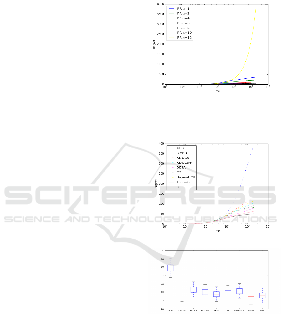
First, a simulation is carried out to ﬁnd out the best

value for parameter α to be used in the PR method,

see Fig. 3. α = 8 is identiﬁed as the best value and

used for this scenario 1. Note that in DPR, no previ-

ous knowledge regarding the scenario is required.

Now, the 50,000 simulations with 20,000 itera-

tions each are carried out. Fig. 4 shows the evolu-

tion of the regret for the different allocation strate-

gies under comparison along the 20,000 iterations

corresponding to one simulation (using a logarithmic

scale), whereas Fig. 5 shows the multiple boxplot cor-

responding to regrets throughout the 50,000 simula-

tions.

The ﬁrst two columns in Table 1 show the mean

regrets and standard deviations for the policies. The

three with lowest mean regrets are highlighted in bold,

corresponding to DPR, PR and BESA, respectively.

The variance is similar for all the policies under con-

sideration. It is important to note that although PR

Figure 3: Selecting parameter α for PR in scenario 1.

(α = 8) slightly outperforms DPR, DPR requires nei-

ther previous knowledge nor a simulation regarding

the arm distributions, which makes DPR more suit-

able in a real environment.

Figure 4: Policies in one simulation for scenario 1,

Figure 5: Multiple boxplot for policies in scenario 1.

Note that in the above multiple boxplots negative

regret values are displayed. It could be considered

an error at ﬁrst sight. The explanation is as follows:

the optimum expected reward µ

∗

used to compute re-

grets is the theoretic value from the distribution, see

Eq. (1). For instance, in an arm with Bernoulli distri-

bution with parameter 0.1, µ

∗

after n plays is 0.1 × n.

However, in the simulation the number of success if

the arm is played n times may be higher than this

ICORES 2017 - 6th International Conference on Operations Research and Enterprise Systems

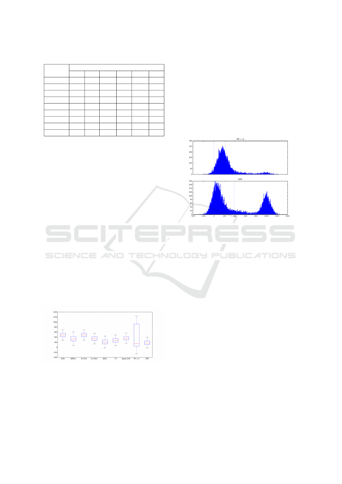
Table 1: Statistics in scenarios 1, 2 and 3.

Bernoulli (low) Bernoulli (med) Bernoulli (G)

Mean σ Mean σ Mean σ

UCB1 393.7 57.6 490.9 104.9 2029.1 125.9

DMED+ 83.1 46.1 356.8 151.5 889.8 313.2

KL-UCB 130.7 47.9 491.5 104.3 1169.6 233.2

KL-UCB+ 103.3 46.0 349.7 104.7 879.7 254.5

BESA 78.1 53.9 281.6 260.9 768.75 399.2

TS 91.1 45.6 284.2 125.1 - -

Bayes-UCB 115.1 46.6 366.3 104.5 - -

PR 51.1

∗

49.2 380.5 426.2 431.0

∗

383.5

DPR 63.6 49.1 214.6

∗

185.1 643.0 387.1

amount, overall in the ﬁrst iterations, leading to nega-

tive regret values.

4.2 Scenario 2: Bernoulli Distribution

and Medium Expected Rewards

In this scenario, we still consider a Bernoulli distri-

bution but now parameters are very similar in the 10

arms and close to 0.5. This leads to the greatest vari-

ances in the distributions, where in almost all arms in

half of the cases they have a value 1 and 0 in the other

half. Thus, it becomes harder for algorithms to reach

the optimal solution. Moreover, if an intensive search

is not carried out along a sufﬁcient number of iter-

ations, we could easily reach sub-optimal solutions.

The parameters for the 10 arms under consideration

are: [0.5, 0.45, 0.45, 0.45, 0.45, 0.45, 0.45, 0.45, 0.45,

0.45].

First, a simulation was carried out again to ﬁnd

out the best value for parameter α to be used in the

PR method in this scenario and α = 2 was selected.

In Fig. 6 the regrets throughout the 50,000 simula-

tions corresponding to the different policies are shown

by means of a multiple boxplot.

Figure 6: Multiple boxplot for policies in scenario 2.

It draws to attention the high variability on the re-

gret values for the PR method (α = 2). Fig. 7 shows

the histograms corresponding to PR (α = 2) and DPR.

As expected, regret values are mainly concentrated

close to value 0 and around value 1000. Note that

the success probability is 0.45 in 9 out of the 10 arms,

whereas it is 0.5 for the other one. The probability

difference is then 0.05 and as the reward is 1 (if suc-

cessful) and 20,000 iterations are carried out, we ex-

pect regret values around value 1000.

The dotted vertical lines in the histograms repre-

sent the regret value 0 and the mean regret throughout

the 50,000 simulations. Note that the mean regret for

PR is not representative. The number of regret obser-

vations around the value 1000 is considerably higher

for PR than DPR, which explains the higher standard

deviation in PR and demonstrates that DPR outper-

forms PR in this scenario.

Figure 7: Histograms for PR (α = 2) and DPR in scenario

The three allocation strategies with lowest aver-

age regrets, highlighted in bold in the third and fourth

columns in Table 1, corresponds to DPR, BESA and

TS, respectively. However, DPR outperforms BESA

and TS, whose performances are very similar but

BESA has a higher variability.

4.3 Scenario 3: Bernoulli Distribution

and Gaussian Rewards

In this scenario, Bernoulli distributions with very low

expected rewards (about 1% success ratios) are again

considered but now rewards are not 0 or 1, they are

normally distributed. This scenario has never been

considered in the literature but we consider it inter-

esting for analysis. We can also face this scenario in

on-line marketing and digital advertising. As in sce-

nario 1, advertising is displayed in banner spaces and

in case the customer clicks on the banner then s/he is

redirected to the page that offers the product. How-

ever, in this new scenario the customer may buy more

than one product, the number of which is modeled by

a normal distribution.

The success ratios in these campaigns are usually

quite low, as in scenario 1, being about 1%. For this,

the ten arms will be used with a Bernoulli distribution

The Possibilistic Reward Method and a Dynamic Extension for the Multi-armed Bandit Problem: A Numerical Study

and the following parameters: [0.1, 0.05, 0.05, 0.05,

0.02, 0.02, 0.02, 0.01, 0.01, 0.01]. Besides, the same

σ = 0.5 is used for the normal distributions, whereas

the following means (µ) are considered: [1, 2, 1, 3,

5, 1, 10, 1, 8, 1]. Moreover, all rewards are truncated

between 0 and 10. Thus, the expected rewards for the

ten arms are [0.1, 0.1, 0.05, 0.15, 0.1, 0.02, 0.2, 0.01,

0.08, 0.01], and the seventh arm is the one with the

highest expected reward.

TS and Bayes-UCB policies are not analyzed in

this scenario since both cannot be applied. α = 70 will

be used in the PR method. Fig. 8 shows the multiple

boxplot for the regrets throughout the 50,000 simula-

tions, whereas the mean regrets and the standard de-

viations are shown in last two columns of Table 1.

The three policies with lowest mean regrets, high-

lighted in bold in Table 1, correspond to PR, DPR and

BESA, respectively, the three with a similar variabil-

ity. However, PR outperforms DPR and BESA in this

scenario.

Figure 8: Multiple boxplot for policies in scenario 3.

4.4 Scenario 4: Truncated Poisson

Distribution

A truncated in [0,10] Poisson distribution is used in

this scenario. It is useful to model real scenarios

where the reward depends on the number of times

an event happens or is performed in a time unit, for

instance, the number of followers that click on the

”like” button during two days since it is uploaded.

The values for parameter λ in the Poisson distribution

for each arm are: [0.75, 1, 1.25, 1.5, 1.75, 2, 2.25].

The variant kl-poisson-UCB was also considered

for analysis, whereas TS and Bayes-UCB will no

longer be considered since both cannot be applied in

this scenario.

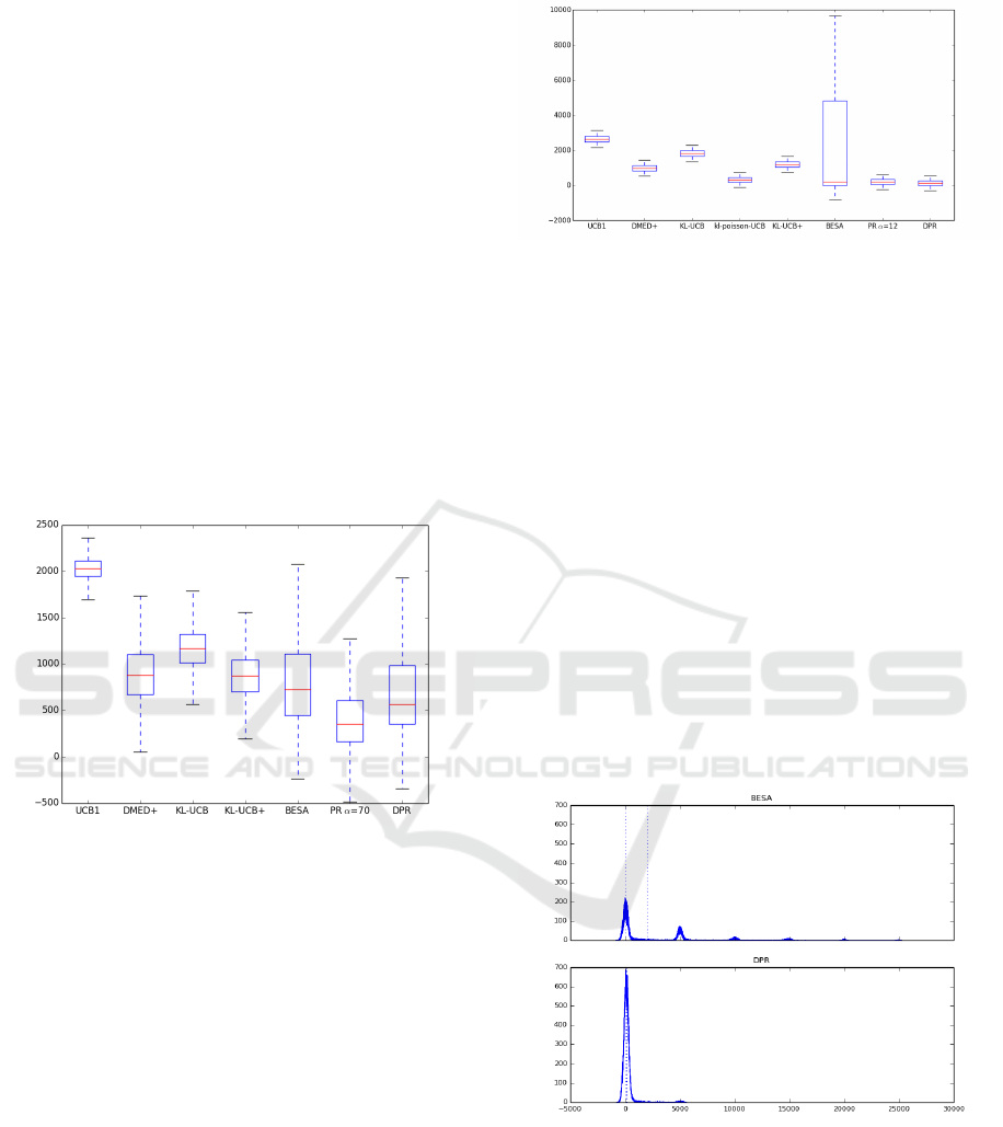
First, the selected value for parameter α to be used

in the PR method in this scenario is 12. Fig. 9 shows

the multiple boxplot for the regrets throughout the

50,000 simulations, whereas the ﬁrst two columns in

Figure 9: Multiple boxplot in the fourth scenario (Poisson).

Table 2 show the mean regrets and standard devia-

tions.

One should observe the high variability on the re-

gret values in BESA. Fig. 10 shows the histograms

corresponding to BESA and DPR. As expected, re-

gret values are mainly concentrated around 7 values

(0, 5000, 10,000, 15,000, 20,000, 25,000, 30,000),

with the highest number of regret values around 0,

followed by 5000 and so on. Note that the different of

λ values in the 7 arms is 0.25 and 0.25 × 20, 000 iter-

ations carried out in each simulation is 5000, which

matches up with the amount incremented in the 7

points the regrets are concentrated around.

The number of regret observations around the

value 0 regarding the remaining values is consider-

ably higher for DPR than BESA, which explains a

higher standard deviation in BESA and demonstrates

that BESA is outperformed by the other policies in

this scenario.

Figure 10: Histograms for BESA and DPR.

DPR again outperforms the other algorithms on

the basis of the mean regrets, including PR (α = 12),

see Table 2. kl-poisson-UCB Poisson is the only pol-

icy whose results are close to DPR and PR. However,

the variability in DPR is higher than in all the other

policies apart from BESA.

ICORES 2017 - 6th International Conference on Operations Research and Enterprise Systems

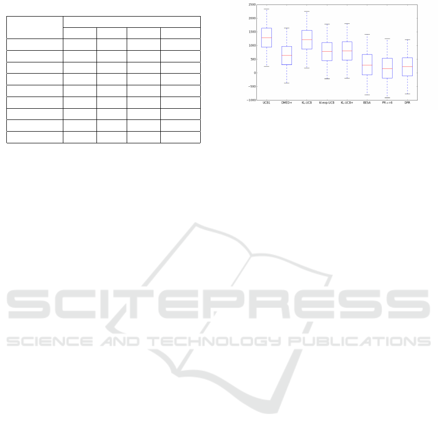
Table 2: Statistics in scenarios 4 and 5.

Truncated Poisson Truncated Exponential

Mean σ Mean σ

UCB1 2632.65 246.03 1295.79 514.03

DMED+ 978.56 225.24 645.70 493.8

KL-UCB 1817.4 236.57 1219.98 510.69

kl-poisson-UCB 314.99 201.79 - -

KL-exp-UCB - - 786.30 498.16

KL-UCB+ 1190.64 225.82 813.45 494.59

BESA 2015.73 3561.5 755.87 2323.22

PR 196.24 212.45 580.31 2182.02

DPR 153.3

∗

409.17 282.83

∗

814.72

4.5 Scenario 5: Truncated Exponential

Distribution

A truncated exponential distribution is selected in this

scenario, since it is usually used to compare alloca-

tion strategies in the literature. It is used to model

continuous rewards, and for scales greater than 1 too.

Moreover, it is appropriate to model real situations

where the reward depends on the time between two

consecutive events, for instance, the time between a

recommendation is offered on-line until the customer

ends up buying. The values for parameter λ in the ex-

ponential distribution for each arm are: [1, 1/2, 1/3,

1/4, 1/5, 1/6].

The variant kl-exp-UCB was incorporated into the

analysis in this scenario, whereas TS and Bayes-UCB

cannot be applied.

The best value for parameter α for the PR method

is 6. Fig. 11 shows the multiple boxplot for the re-

grets throughout the 50,000 simulations. The mean

regret and the standard deviations are shown in last

two columns of Table 2.

PR and DPR again outperform the other policies,

with PDR being very similar to but slightly better than

PR in this scenario. Moreover, DPR requires neither

previously knowledge nor a simulation of the arm dis-

tributions, what makes DPR more suitable in a real

environment. The best four policies are the same as

in scenario 4, with a truncated Poisson, changing the

KL-poisson-UCB with KL-exp-UCB.

5 CONCLUSIONS

In this paper we propose a novel allocation strategy,

the possibilistic reward method, and a dynamic ex-

tension for the multi-armed bandit problem. In both

methods the uncertainty about the arm expected re-

wards are ﬁrst modelled by means of possibilistic re-

Figure 11: Multiple boxplot for policies in the ﬁfth sce-

nario.

ward distributions derived from a set of inﬁnite nested

conﬁdence intervals around the expected value. Then,

a pignistic probability transformation is used to con-

vert these possibilistic function into probability dis-

tributions. Finally, a simulation experiment is carried

out by sampling from each arm to ﬁnd out the one

with the highest expected reward and play that arm.

A numerical study suggests that the proposed

method outperforms other policies in the literature.

For this, ﬁve complex and representative scenarios

have been selected for analysis: a Bernoulli distribu-

tion with very low success probabilities; a Bernoulli

distribution with success probabilities close to 0.5,

which leads to the greatest variances in the distribu-

tions; a Bernoulli distribution with success probabili-

ties close to 0.5 and Gaussian rewards; a truncated in

[0,10] Poisson distribution; and a truncated in [0,10]

exponential distribution.

In the ﬁrst three scenarios, in which the Bernoulli

distribution is considered, PR or DPR are the policies

with the lowest mean regret and with similar variabil-

ity regarding the other policies. BESA is the only pol-

icy with results that are close to DPR and PR, mainly

in scenario 1. Besides, DPR and PR clearly outper-

form the other policies in scenarios 4 and 5, in which

a truncated Poisson and exponential are considered,

respectively. In both cases, DPR outperforms PR.

ACKNOWLEDGEMENTS

The paper was supported by the Spanish Ministry

of Economy and Competitiveness MTM2014-56949-

C3-2-R.

REFERENCES

Agrawal, R. (1995). Regret bounds and minimax policies

under partial monitoring. Advances in Applied Prob-

ability, 27(4):1054–1078.

The Possibilistic Reward Method and a Dynamic Extension for the Multi-armed Bandit Problem: A Numerical Study

Audibert, J.-Y. and Bubeck, S. (2010). Sample mean based

index policies by o(log n) regret for the multi-armed

bandit problem. Journal of Machine Learning Re-

search, 11:2785–2836.

Audibert, J.-Y., Munos, R., and Szeperv

ari, C. (2009).

Exploration-exploitation trade-off using variance esti-

mates in multi-armed bandits. Theoretical Computer

Science, 410:1876–1902.

Auer, P., Cesa-Bianchi, N., and Fischer, P. (2002). Finite-

time analysis of the multiarmed bandit problem. Ma-

chine Learning, 47:235–256.

Auer, P. and Ortner, R. (2010). UCB revisited: Improved

regret bounds for the stochastic multi-armed bandit

problem. Advances in Applied Mathematics, 61:55–

65.

Baransi, A., Maillard, O., and Mannor, S. (2014). Sub-

sampling for multi-armed bandits. In Proceedings

of the European Conference on Machine Learning,

page 13.

Berry, D. A. and Fristedt, B. (1985). Bandit Problems:

Sequential Allocation of Experiments. Chapman and

Hall, London.

Burnetas, A. N. and Katehakis, M. N. (1996). Optimal

adaptive policies for sequential allocation problems.

Advances in Applied Mathematics, 17(2):122 – 142.

Capp

e, O., Garivier, A., Maillard, O., Munos, R., and Stoltz,

G. (2013). Kullbackleibler upper conﬁdence bounds

for optimal sequential allocation. Annals of Statistics,

41:1516–1541.

Chapelle, O. and Li, L. (2001). An empirical evaluation of

thompson sampling. In Advances in Neural Informa-

tion Processing Systems, pages 2249–2257.

Dubois, D., Foulloy, L., Mauris, G., and Prade, H.

(2004). Probability-possibility transformations, trian-

gular fuzzy sets, and probabilistic inequalities. Reli-

able Computing, 10:273–297.

Dupont, P. (1978). Laplace and the indifference principle in

the ’essai philosophique des probabilits.’. Rendiconti

del Seminario Matematico Universit e Politecnico di

Torino, 36:125–137.

Garivier, A. and Capp

e, O. (2011). The kl-ucb algorithm

for bounded stochastic bandits and beyond. Technical

report, arXiv preprint arXiv:1102.2490.

Gittins, J. (1979). Bandit processes and dynamic alloca-

tion indices. Journal of the Royal Statistical Society,

41:148–177.

Gittins, J. (1989). Multi-armed Bandit Allocation Indices.

Wiley Interscience Series in Systems and Optimiza-

tion. John Wiley and Sons Inc., New York, USA.

Hoeffding, W. (1963). Probability inequalities for sums

of bounded random variables. Advances in Applied

Mathematics, 58:13–30.

Holland, J. (1992). Adaptation in Natural and Artiﬁcial Sys-

tems. MIT Press/Bradford Books, Cambridge, MA,

USA.

Honda, J. and Takemura, A. (2010). An asymptotically op-

timal bandit algorithm for bounded support models. In

Proceedings of the 24th annual Conference on Learn-

ing Theory, pages 67–79.

Kaufmann, E., Capp

e, O., and Garivier, A. (2012). On

bayesian upper conﬁdence bounds for bandit prob-

lems. In International Conference on Artiﬁcial Intel-

ligence and Statistics, pages 592–600.

Lai, T. and Robbins, H. (1985). Asymptotically efﬁcient

adaptive allocation rules. Advances in Applied Math-

ematics, 6:4–22.

Maillard, O., Munos, R., and Stoltz, G. (2011). Finite-

time analysis of multi-armed bandits problems with

kullback-leibler divergences. In Proceedings of the

24th Annual Conference on Learning Theory, pages

497–514.

Smets, P. (2000). Data fusion in the transferable belief

model. In Proceedings of the Third International Con-

ference on Information Fusion, volume 1, pages 21–

33.

Sutton, R. S. and Barto, A. G. (1998). Introduction to Re-

inforcement Learning. MIT Press, Cambridge, MA,

USA, 1st edition.

ICORES 2017 - 6th International Conference on Operations Research and Enterprise Systems