
Visual Interactive Creation of Geo-located Networks
Felix Brodkorb
1
, Manuel Kopp
1
, Arjan Kuijper
2
and Tatiana von Landesberger
1
1
TU Darmstadt, Darmstadt, Germany
2
Fraunhofer IGD, Darmstadt, Germany
Keywords:
Geographic Networks, Graph Generators, Graph Editors.
Abstract:
Nodes in real world networks often have a geographic position. In many cases such as for simulation or op-
timization, there is a need for non-trivial synthetic geo-located networks. As synthetic datasets are required
to have specific properties such as connectivity and geographic distribution, often networks need to be gener-
ated. However, their creation is cumbersome if done purely by hand, and inflexible if done fully automated.
Here, we present a framework for creating artificial geographic located networks in a visually interactive way.
We designed our framework with the what-you-see-is-what-you-get principle in mind, i.e. showing the (in-
termediate) results of the interactive creation process at any time and allowing the user to adjust the network
iteratively. This design allows our system to be also used as a simple viewer for networks that have incomplete
location information. Our approach consists of two steps: (1) Creating the network topology and (2) assigning
locations to its nodes. Our half automatic system enables the user to easily set the location of the nodes to pre-
defined areas like countries, states, and urban regions, while still being able to flexibly and interactively control
the creation process. We show the utility of our system by creating a real-world-like geo-located network.
1 INTRODUCTION
Many networks in real life have a geographic loca-
tion attached to their elements. For example computer
networks like backbones of the companies AT&T and
NTT consists of computers (nodes) that have a phys-
ical location. Other networks with geographic loca-
tion exist, like delivery network, friendship networks,
transportation networks, or collaboration networks.
Such networks are used in business and research and
have a geographic relation that is often abstracted
from.
However, geographic context is relevant as might
influence rationales and decisions. Additionally, ge-
ographic context is not necessary retrieved directly
from the topology of the network and can be – in the
worst case – entirely independent of it. For exam-
ple, two nodes in a supply chain network can be sepa-
rated by a national border, resulting in additional pro-
cedures such as customs. Many other types of back-
ground knowledge might be relevant (e.g. culture, cli-
mate, or jurisdiction).
Synthetic geo-located network data is necessary
for analysis, simulation or optimization of networks.
Beside general geo-located network data, network
data with use-case dependent geographic properties is
required for testing of algorithms or approaches. Ad-
ditionally, researchers need to create multiple, slightly
similar networks for studies and evaluations. How-
ever, real world data is difficult to obtain, and geo-
based networks are cumbersome to create manually.
Manual creation is especially cumbersome when one
wants to have multiple networks that differ only in
defined parts that can not usually be found in the real
word.
Graphs or networks are a common element used
for visual analytics. In this paper, we use the terms
“graph” and “network” interchangeably. For an
overview of graph visualization possibilities, we re-
fer to (von Landesberger et al., 2011). Visual analyt-
ics approaches visualize the graph structure and de-
tect special parts or sections in a wide range of ap-
plication areas (von Landesberger et al., 2009; von
Landesberger et al., 2013). Here we summarize the
most relevant aspects of geo-located graphs. A graph
G(V, E) consists of vertices V and vdges E. An edge
e ∈ E connects two vertices v
i
, v
j
∈ V . A graph whose
edges are directed is called a directed graph. Vertices
and edges can have attributes. If vertices and/or edges
have attributes that represent locations on earth, one
has a geo-located graph. Here, we focus on networks
where only vertices have a geographic location.
In this paper, we present a framework for creat-
Brodkorb F., Kopp M., Kuijper A. and von Landesberger T.
Visual Interactive Creation of Geo-located Networks.
DOI: 10.5220/0006176302830293
In Proceedings of the 12th International Joint Conference on Computer Vision, Imaging and Computer Graphics Theory and Applications (VISIGRAPP 2017), pages 283-293
ISBN: 978-989-758-228-8
Copyright
c
2017 by SCITEPRESS – Science and Technology Publications, Lda. All rights reserved
283

ing geo-located networks or attaching geographic lo-
cation information to an existing network. The frame-
work aims to improve the manual creation process.
With our approach, we cover two generic scenarios:
1. Create a network topology from scratch and add
location information to its nodes.
2. Import a network topology and add location infor-
mation to its nodes.
To reach this goal, we mainly introduce the following
approaches:
• An interactive and iterative visual workflow.
• Implementation of the what-you-see-is-what-you-
get (WYSIWYG) principle to show the current
network after each operation.
• Concurrent visualization of mixed networks that
contain nodes with and without geographic infor-
mation at the same time.
• Assign many nodes to hierarchic geographic areas
in the world at any scale.
Using the framework, a user can quickly create geo-
located networks with hundred of nodes while still
having control over the locations of its nodes. We
focus on the interactive visual creation process and
leave techniques that aim at the recreation of statis-
tical features of more specific types of geo-networks
for future work. While designing our system, we tried
to keep it’s usability as simple and straight forward as
possible by for example avoiding things like multi-
ple views and dialogs. To the best of our knowledge,
there are no approaches by now that generate artificial
geographic networks in an interactive way. Addition-
ally, we found out that our system is also useful as
a simple viewer for networks that contain nodes with
and nodes without location information at the same
time (mixed networks).
This paper is structured as follows: Section 2
shows related work about geo-located networks and
graph generation. Section 3 presents our approach in
detail. In Section 4, we show a usage example by
trying to mimic a real-world network. Section 5 dis-
cusses the limits of our approach. Finally, Section 6
concludes this paper and outlines future work.
2 RELATED WORK
In research, the creation of synthetic datasets is an
important topic, e.g. for testing algorithms. Man-
ual data creation is very cumbersome, so automatic
and interactive visual systems have been developed.
A number of approaches exist that create data of
a specific type (e.g. multivariate data (Albuquerque
et al., 2011; Bremm et al., 2012; Wang et al., 2013),
scenario-based data (Whiting et al., 2008), and syn-
dromic surveillance data (Maciejewski et al., 2009)).
We focus on geographic network data.
Geographic data is usually gained by sensor sys-
tems, collected by surveys or generated using spatio-
temporal patterns (Theodoridis et al., 1999; Sak-
shaug and Raghunathan, 2010; Sakshaug and Raghu-
nathan, 2014a). Our previous work (Brodkorb et al.,
2016) shows an rule-based approach that generates
tree-shaped geo-located network data. It focuses on
tree-shaped networks and also has the drawback that
the creation process is controlled by general purpose
graphical user interface (GUI) controls, like list-views
or edit fields that don’t allow visual parameter manip-
ulation. To the best of our knowledge, all other exist-
ing geographic data generators do not create network
structures, but solely produce data on a predefined
geographic grid (e.g., (Sakshaug and Raghunathan,
2014b)). Some approaches use existing transporta-
tion networks as a basis (Frick, 2011; Cascetta and
Cantarella, 1993; Brinkhoff, 2002), but do not cre-
ate new network structures with geographic locations
in a visually interactive way. SANET (Okabe et al.,
2006a; Okabe et al., 2006b) generates random points
ontop of an existing geo-located network. Further,
there are approaches that focus on the creation of city
structures such as street networks (Parish and M
¨
uller,
2001; Chen et al., 2008). However, these networks
represent a very specific geographically located net-
work, since they have a quite regular structure when
compared to other types of networks.
Graph generation systems can be categorized
into (1) algorithmic and (2) visualization-based ap-
proaches:
2.1 Algorithmic Approaches
Algorithmic graph generators produce graphs that
are automatically based on input parameters (e.g.,
(Brinkmann and McKay, 2007; Ying and Wu, 2009)).
Parameter-based generation is not well suited to con-
trol graph generation in a visual way and to edit it
interactively. Most close to our work are (Baeza-
Yates et al., 2010) and (
´
Alvarez-Garc
´
ıa et al., 2014;
Alvarez-Garcia et al., 2012) which use a set of rules
for generating graphs. However, these approaches
were designed to extract graphs from arbitrary data
and not to generate new graphs without any input
datasets. Moreover, they do not provide the possibil-
ity to generate geo-locations of nodes together with
a graph structure. Beside these generators, the auto-
Poisson model (Griffith, 2002) can be used to gener-
IVAPP 2017 - International Conference on Information Visualization Theory and Applications
284
ate geographic structures. However, it has no visual
way to control the creation process.
2.2 Visualization-based Approaches
Visual graph editors take an interactive approach.
They enable the user to steer the creation process. As
many interactive graph editing projects have shown
(O’Madadhain et al., 2003; YWorks, 2015; Wong
et al., 2006; Benson, 2015; Spritzer and Freitas, 2008;
McGuffin and Jurisica, 2009; Gladisch et al., 2014),
techniques for direct and interactive manipulation of
datasets (Baudel, 2006) can be performed on graphs.
In such projects, the user has to edit node and edge
separately. Editing single nodes and edges obviously
do not scale for bigger graphs. yED (YWorks, 2015)
and Illuminations (National Council of Teachers of
Mathematics, 2015) use pre-defined graph templates
to create graphs where the size of the graph can be ad-
justed by the user. However, they only allow creating
complete graphs. Recently, two interactive systems
were presented which allow for iterative graph gen-
eration in a visual interface coupled with automatic
graph generators: The evolutionary graph generation
algorithm developed by (Bach et al., 2013) iteratively
generates multiple graphs, each with different param-
eters. (von Landesberger et al., 2010) proposed an ap-
proach that enables users to create graphs by combin-
ing pre-defined building blocks interactively. In some
systems, the user can specify attributes for individual
nodes and edges. However, to the best our knowledge,
there is no system other than (Brodkorb et al., 2016)
with the possibility to directly create graphs with a
geographic location following a given geographical
structure.
3 APPROACH
In this section, we propose an interactive visual gener-
ator for geo-networks. As the aim is to use it for test-
ing, analysis, simulation or optimization of the net-
work and algorithms on it, we use inspiration from
interactive graph editing projects (see 2.2). We use
a geographic map as background and place a user-
defined network on it that a user can edit incremen-
tally. Our primary focus was to keep the system sim-
ple to be easy to use, and general to apply to a broad
range of different geo-located networks. Except di-
alogs used to set parameters for the network structure
generators, we designed our system to be used from
a single view only, because with growing amount of
data coordinated multiple views are harder to handle
for computers as well as users (Andrienko and An-
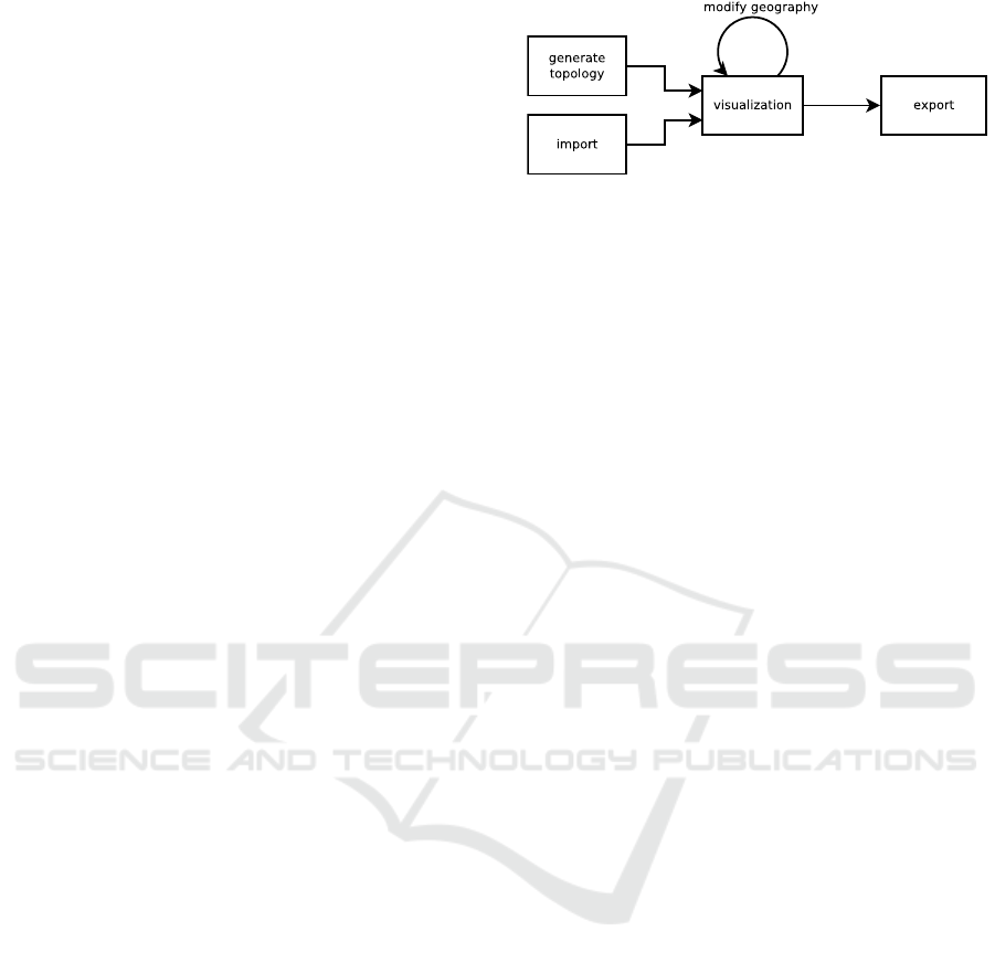
Figure 1: Pipeline showing the workflow of creating geo-
based networks.
drienko, 2007). Please see also the attached video for
a demonstration of the most important techniques pre-
sented in our approach.
Issues that we address in our approach are
• workflow and interaction,
• topology,
• layout issues,
• visual representation,
• assigning geographic information to nodes.
In this approach, we concentrate on the geography
of the nodes of a network that has been either created
or imported. Geography of a network is defined by
attributes that are attached to its nodes. The geogra-
phy of the edges will be defined by the geography of
its endpoint nodes. Because of this, edges contain no
explicit geographic information themselves, and our
system draws them as straight lines between their end-
point nodes.
3.1 Workflow and Interaction
Our pipeline for generating geographic networks con-
sists of two steps (see Figure 1): (1) Generate (or
load) a network topology and (2) assign geographic
information to its nodes.
3.2 Topology
The first step is creating the topology of a network, i.e.
a network structure without geo-information. Topol-
ogy of a network describes which nodes are connected
to each other via edges. Many network features can
be deducted from the topology, like reachability of
one node from another node or hop distance between
two nodes. We target two general use-cases:
1. A user needs to create a geo-located network from
scratch including its topology and
2. a user needs to assign geo-location to an existing
topology.
We support case 1 by supplying generators for
the following topologies: Trajectory, tree, directed
Visual Interactive Creation of Geo-located Networks
285

acyclic graph, interconnected star-shaped networks,
Barab
´
asi scale-free network (Barab
´
asi and Albert,
1999), Erd
¨
os-R
´
enyi random graph (Erd
¨
os and R
´
enyi,
1959), Kleinberg small-world network (Kleinberg,
2000), and Eppstein power-law graph (Eppstein and
Wang, 2002). Alternatively, the user can import an
existing network into the system which targets case 2.
Imported networks may contain (partly) geo-locations
in their nodes. The system does not restrict the type
of network, and there are no restrictions on network
topology for importing graphs. Similar to import-
ing, we support exporting of (partly) geo-located net-
works, too. The focus of our system is assigning geo-
locations to a given network topology. However, we
also provide the user with simple graph editing tech-
niques (i.e. adding, removing and connecting nodes)
that allow modification of the topology.
3.3 Layout
The layout of a network defines the positions of its
nodes on a two-dimensional plane. A large set of lay-
out algorithms has been developed to improve the vi-
sualization of networks (Herman et al., 2000; D
´
ıaz
et al., 2002). For geo-located networks, the layout
is already given by the geo-information in its nodes.
Assigning geographic information to nodes will indi-
rectly influence the layout of the network.
In our approach, we pursuit the WYSIWYG prin-
ciple. By making a WYSIWYG-based system, we
intended to vastly speed up the user’s work process
by preserving him from mental context switching be-
tween other dialogs/views, as well as GUI operations
like (re)opening them. The network - once created or
imported - will be displayed on the map. All further
operations will be done directly in this map view. A
user can see the results of each operation immediately
and revoke, improve or alter them.
During editing, the network will contain a mix
of nodes with and without geo-information. We de-
signed our visualization to show both of these types
of nodes on the same network at the same time (see
Figure 2). Besides showing the network in the state of
being edited, this design can also be used as a simple
viewer to visualize partly geo-located networks. This
technique enables users to look at networks in com-
mon cases like when the location information of one
or a few is simply missing.
Map transformations define the area and scale of
the map that is currently visible for the user. Nodes
with geo-information will be placed on the map at
the corresponding position and directly react to map
transformations. Nodes without geographic informa-
tion don’t have a predefined location. A generic lay-
out algorithm will calculate their locations indepen-
dently of the map transformations. This way, we
can combine a nice looking layout as achieved by
common layout algorithms with a partially fixed geo-
graphic context but still avoiding overplotting.
We also considered other ways of showing mixed
networks: Displaying the nodes without geographic
information at a special location like the screen bor-
der or an off-centered inset makes the layout algo-
rithm inflexible and amplifies clutter. Showing them
at another fixed location on the map or leaving them
completely out gives the user a wrong impression of
the data. Using a geographic view for geo-located
nodes and a non-geographic structural view for all
nodes to show different subviews of a network vio-
lates our WYSIWYG principle and requires frequent
mental task switching from the user.
In the examples shown in this paper, we use spring
layout (Eades, 1984) because it is one of the most fa-
mous force-directed layout algorithms. However, any
other layout algorithm can be used, too, and, depend-
ing on the use-case, improve the visual representation
of the network further.
When changing the layout of nodes, one common
effect is a sudden change of the location of one or
multiple nodes. It looks to the user as if the nodes
are jumping and the user can hardly keep track of
this. Jumping of nodes destroys the user’s mental
map forcing him to review the whole graph and thus
increasing the time spent on the editing task and the
chance of making mistakes. This effect happens when
assigning a location to many nodes supported by our
location assigning algorithm (see Section 3.5). As
stated above, our system allows arbitrary layout al-
gorithms for nodes without location. Even though
spring layout that we mentioned above adjusts node
locations smoothly to avoid sudden jumping of nodes,
other layout algorithms will probably cause sudden
changes in node locations and thus triggering jump-
ing effects.
To avoid jumping effects, we use animation effects
for node position changes: Nodes will not be put im-
mediately to their destination locations but moved to-
ward them with limited speed. This effect gives the
impression of a smooth and fluid animation. Using
this kind of animation has shown to have two addi-
tional advantages:
• The sluggish movement of nodes without location
information makes these nodes react slightly dif-
ferent to map transformations and thus to stand
out. This effect is an additional visual clue be-
side the color-based visual clues that we will show
for the presence/absence of location information
of nodes (see Section 3.4).
IVAPP 2017 - International Conference on Information Visualization Theory and Applications
286
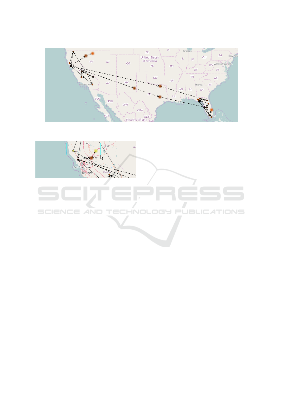
Figure 2: After generating a network, we placed 7 nodes in California and 8 nodes in Florida. Blurred nodes yet have to be
assigned to locations and their layout is calculated by a force directed layout algorithm.
Figure 3: A network with nodes being selected. The yel-
low nodes inside the light blue border are selected while the
orange nodes are not selected.
• The sluggish movement of nodes hides wiggling
effects caused by some race conditions or numer-
ical imprecision of a chosen layout algorithm.
For a better impression of this animation effect, we
refer to our video.
3.4 Visual Representation
The visual representation of a network defines how
nodes and edges are displayed and how their attributes
and properties are visually encoded. In our approach,
we draw nodes as circles. Node color (orange) rep-
resents node degree where darker color means higher
node degree. However, any other information could
be encoded by node color instead (e.g. a given node
attribute). We enable the user to select nodes using a
rectangle tool. Selected nodes are marked by bright
yellow (see Figure 3).
Edges are drawn as straight lines. In the case of
directed edge, an arrow indicates edge direction. We
don’t use edge colors in this context, so this attribute
can be used to visualize other properties.
When a user edits a network there will likely be
the situation where it contains a mix of nodes with
and nodes without location information. Even for a
few nodes, we found out that it is hard for users to
remember which nodes already have location infor-
mation and which do not, especially, when users are
navigating the map. Figure 2 shows a mixed net-
work. Nodes without geo-information will be shown
blurred on the map, while nodes with geo-information
will not be distorted. This way, we intend to create
the impression of unclear location. We distinguish
three types of edges: (1) edges between nodes with
defined locations are solid, (2) edges between nodes
one with and one without defined location are dotted
with thick and long strokes, and (3) edges between
nodes with undefined locations are dotted with light
and short dots. Blurred nodes graphics are precom-
puted in order to speed up visualization. We also in-
tended to blur edges similar to nodes. However, the
edges’ paths (and thus looks) are not static, so a blur-
ring effect has to be computed in real-time for each
edge for each frame. Real-time blurring would have a
bad impact on performance and thus effectively pre-
venting bigger networks from being displayed fluidly.
3.5 Assigning Geographic Information
After a network topology has been created or loaded,
a user can start to attach geography to its nodes.
Assigning locations on a node-by-node basis is
very cumbersome as the time to place the nodes of
a network depends linearly on the number of nodes.
However, pure automatic placement has the disadvan-
tage that the user has no control over the placement of
the nodes. We want to provide the user with a system
that enables the user to place an arbitrary number of
nodes automatically.
In contrast to pure automatic placement, the user
should remain in full control about the area where
nodes will be placed in our system. Further, the sys-
tem should assist by suggesting meaningful areas. On
Visual Interactive Creation of Geo-located Networks
287

the other hand, we want to preserve as much free-
dom as possible, so that our system can be applied
not only to some specific networks but general geo-
located networks.
To propose meaningful areas, we use a database-
based approach. A database provides a set of areas
that the system will use for placement of nodes. The
database we use in our examples contains the admin-
istrative subdivision of the world because the political
division is commonly known and often implies impor-
tant information when looking at geo-data. This infor-
mation might, for example, indicate a change in ad-
ministrative responsibility or applicable laws in case
of a service-based network. Because of this, the struc-
ture of many networks is influenced by political bor-
ders.
However, the database is not limited to adminis-
trative subdivision and can define any subdivision of
the world. Using this exchangeable database-based
approach, we make sure that the system remains flex-
ible in defining what a meaningful area means to the
user.
Depending on the task at hand, it might be nec-
essary to create networks that are on either a big or
small geographic scale. Further, a task might require
the user to create a network that is partly on big and
partly on a small geographic scale at the same time.
Thus, we designed the system to be able to work with
hierarchic area databases. In this kind of database,
the area subdivision forms a tree. We enabled the
user to be able to adjust the active layer of the tree
used for positioning. By changing the active layer,
the user can set the geographic scale of the subdivi-
sion of the world. In the case of our example database,
this means navigating from the subdivision into coun-
tries up to subdivision into cities. Adjusting the geo-
graphic scale will work only if the database contains
hierarchic data. This semi-automated approach helps
to keep the balance between placing nodes in a par-
ticular region and saving the overhead of caring about
details of placement.
Nodes can be assigned to an area using a drag-
and-drop operation. Figure 4 shows how a single node
is dragged by the mouse cursor and dropped to a city
to set its location. While dragging multiple nodes, the
predefined geographic area under the cursor will be
highlighted by an animated dashed border (see Fig-
ure 5a). An animated red border highlights the shape
of the area notably without cluttering the view. High-
lighting gives instant feedback about the size of the
area in which the nodes can be placed. Additionally,
a label will display the area’s name. As mentioned
above, the scale of the area is dependent on the chosen
hierarchy level and can be adjusted freely, even while
dragging. Immediate feedback from the area’s bor-
ders and the label enable the user to select the area of
interest quickly and accurately. When the user drops
the nodes into an area, geo-location within this area
will be assigned to each node (see Figure 5b).
Node placement within an area is calculated by a
coordinate generator algorithm. Like for the database,
we want our system to apply to various kind network
generation tasks, so we designed it to be easily exten-
sible to various coordinate generator algorithms. In
the examples presented here, we use a simple random
coordinate generator that draws two random numbers
(x and y) from interval [0 − 1) and transforms them
into the bounding box area of the shape. A hit-test
makes sure that the coordinate is in contained within
the shape before transforming them to geographical
coordinates. However, depending on the use-case, a
more sophisticated algorithm can be used.
Area shapes are stored in a database. For each
area, the database contains three shapes per area:
• A shape of the area in full resolution used for ac-
tual coordinate generation. When the user drops a
set of shapes into an area, these shapes are used as
boundaries in which the coordinates of the nodes
will be generated.
• A low-resolution shape used for efficient visual-
ization of the area’s borders. This shape is used
for efficient displaying of the area’s borders on
the map. Full resolution shapes often have a
much higher resolution as necessary for display-
ing. This might have a negative impact on ren-
dering performance while not increasing the qual-
ity of the visual result. A user can also use low-
resolution shapes for the actual generation of co-
ordinates to speed up the layout process if he
doesn’t care about the exactness of the layout
around the borders.
• A bounding box used to speed up the point-in-
shape test. This, again, speeds up the rendering,
since, on fine-grained administrative levels, the
number of shapes to check for intersection can be-
come very high.
Since area shapes are immutable, low-resolution
shapes and bounding boxes the bounding boxes have
been pre-calculated.
Borders of administrative areas often include
coast regions. To prevent nodes from being placed
into an ocean, we do not use the administrative
area directly but an intersection of the area with the
world’s land mass. Since this intersection is static, it
has been precomputed and already applied to all full
resolution shapes in the database. However, the in-
tersection has not been applied to the low-resolution
IVAPP 2017 - International Conference on Information Visualization Theory and Applications
288
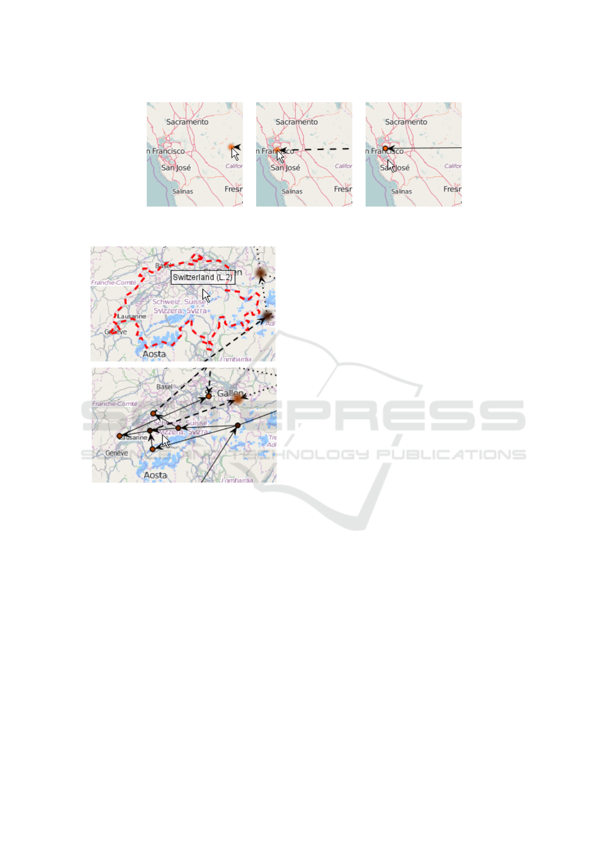
Figure 4: A single node’s location can be assigned directly to a location by dragging it there. The node is selected with the
cursor (left), moved to the intended location (middle), and is dropped there (right) to assign it to this location.
(a)(a)
(b)(b)
Figure 5: (a) Switzerland is highlighted by a dashed border
when the mouse cursor is dragging a set of nodes over it. (b)
After dropping a set of 7 nodes on Switzerland, the system
assigns random coordinates to the nodes within the area of
Switzerland.
shapes used for displaying the borders on the map.
We decided so because many small islands at the coast
lead to visualization artifacts of the marker borders.
4 USAGE EXAMPLE
In this section, we show a concrete example of our
approach by imitating a real network. The exam-
ple we use here is an academic computer network
named “LitNet” located in Lithuania. The dataset was
obtained from http://topology-zoo.org and resembled
the networks in 2009. The network consists of 43
nodes and 43 edges. Figure 6a shows the network
visualized by our tool.
We notice that location information of 4 nodes
in the dataset is missing since our tool shows them
blurred.
Looking at the network, we see that there are 5
nodes (hub nodes) that are forming a cycle. The re-
maining nodes (we call them child nodes) connect
mostly to their nearest hub node, but not to any other
nodes.
To imitate LitNet, we start by creating its topol-
ogy. We use the generator for inter-connected star
networks with 5 hub nodes and 9 nodes per hub (50
nodes in total). Figure 7a shows the resulting net-
work.
Force directed layouting places child nodes near
to their associated hubs. One by one, we drag the
hubs to the rough locations where the real LitNet also
shows hubs. This results in Figure 7b. Next, we con-
tinue by assigning locations to the child nodes of the
hubs, so that they are roughly located near to their
hubs. To do so, we select the child nodes and drag
the selected nodes to the area around the hub node.
The county around the hub node gets highlighted. As
we drop the selected nodes, they will be placed ran-
domly within the county. Figure 7c shows the result
of assigning locations to all child nodes. We edited
the graphic of Figure 7c to be able to show all county
borders in which we placed nodes. In the original data
of LitNet, a few nodes stand out that are unusually far
away from their associated hub. To imitate this aspect,
we drag some random child nodes around the corre-
sponding hub to the positions we see in the original
data. Figure 7d shows the final result of our synthetic
network. We can now export this network and use it
for testing or analysis.
Figure 6 shows the original LitNet and our gen-
erated network side-by-side. We can see how simi-
lar the result looks to the original network. In total,
we used 16 placement operations to imitate LitNet (5
for hubs + 5 for hubs’ child nodes + 6 for individual
nodes). Without our tool, it would have been neces-
sary to adjust each single node resulting in at least 43
operations. By using semi-automated operations, we
could balance between speed and geographic accu-
Visual Interactive Creation of Geo-located Networks
289
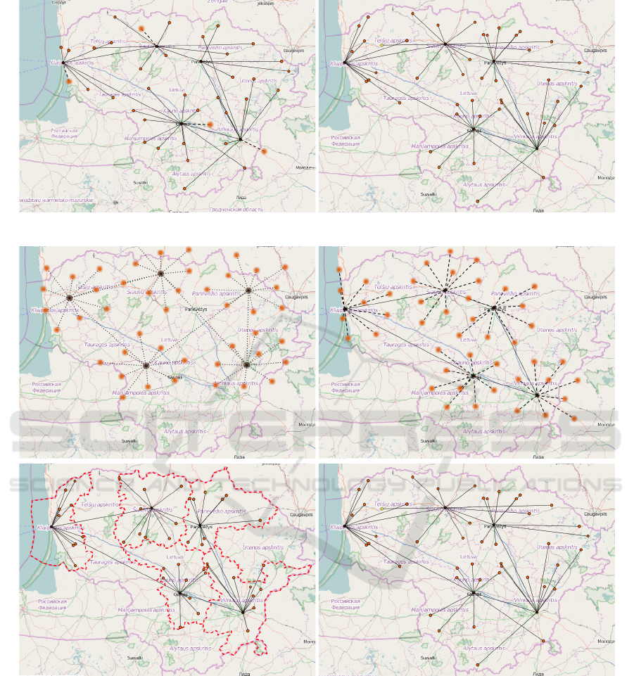
(a) Original LitNet(a) Original LitNet (b) Our Imitation(b) Our Imitation
Figure 6: (a) Original LitNet and (b) the network we created with our tool to imitate LitNet.
(a) No geo-location(a) No geo-location (b) Hubs assigned(b) Hubs assigned
(c)(c)
Child nodeChild node
assignedassigned
(d)(d)
Single nodesSingle nodes
adjustedadjusted
Figure 7: Process of creating a network that resembles LitNet (see Figure 6). (a) The topology of a hub network with star like
topology has been created. (b) Hub nodes of the network have been assigned to locations. (c) Child nodes have been assigned
to the area around their hub node. Their exact location was generated randomly. (Note that the graphic was edited with an
image processor to show the red borders of all the counties in one graphic.) (d) Single nodes have been relocated manually to
make the generated network have similar anomalies like the original network.
racy and incrementally increase the (task dependent)
data quality.
We refer to our attached video for a better visual
demonstration of recreating “LitNet”.
5 DISCUSSION
We have shown how our framework can be used to
attach location information to nodes of a network.
Since we provide a flexible way of assigning a loca-
tion to nodes, our approach can be efficiently used
IVAPP 2017 - International Conference on Information Visualization Theory and Applications
290

not only for small, but also for bigger networks with
hundreds of nodes. However, as the visualization
uses node-link representation, the approach can not be
used effectively to edit large networks with ten thou-
sands or hundred thousands of nodes.
Our algorithm assigns locations to nodes within a
shape in a random way. This behavior is sufficient
if one only wants to create a roughly geographic bal-
anced network. However, depending on the use-case,
one can extend the framework by a custom plug-in for
custom layout calculation within a shape.
As mentioned in Section 3, we used a pre-
calculated intersection of the area shapes with the
landmass for geography generation. This calculation
can be easily extended to include lakes, rivers or un-
populated areas in this operation if required by the use
case.
While all actions can be performed via descrip-
tive menu items, the primary focus of the system is to
perform all actions with mouse and keyboard only to
speed up the editing process once a user got used to
this.
The examples shown in this paper used the recur-
sive administrative division of the world for assign-
ing locations to multiple nodes because they are com-
monly known and accepted, and for many real world
problems, administrative borders are relevant. How-
ever, our approach can be used for any other type of
division of the earth, regardless of whether it is recur-
sive or not. Examples include biospheres of animals
or nautical zones.
All operations in our framework except for layout
calculation operate in O (n) (n = node count). Perfor-
mance mainly depends on the layout algorithm used.
Here, we used a force-directed algorithm that runs
in approximately polynomial time. Assigning geo-
graphic location depends on the number of nodes to
be processed. However, a custom algorithm might
have a different performance depending on the time
complexity of the algorithm used.
Intersection tests on the database of areas test in-
tersection with all shapes of a given hierarchy level.
Since there are many cities and suburbs, we used
bounding boxes to speed up the tests and observed
no noticeable delay anymore. This intersection test
performance can be further improved by using space
subdividing techniques.
Depending on the number of shapes and edges per
shape (data quality), assigning locations to a set of
nodes within an area can be slow. Our system can
speed up the assigning process using simplified ver-
sions of shapes in exchange for accuracy at the bor-
ders. Whether this is acceptable or not depends on
the concrete use-case.
6 CONCLUSION AND OUTLOOK
We presented a framework to create networks with
geolocated nodes. Our approach can be used to eas-
ily and fast create custom geo-located networks. The
framework works interactively and supports incre-
mental refinement following the WYSIWYG princi-
ple. It allows the user to place nodes in an arbitrary
area at any scale by using semi-automated placement
algorithms. Still, a user can edit details such as single
nodes or small groups of nodes. Finally, we showed
that our system could be used to mimic existing geo-
located networks easily by recreating a real network.
At the moment, topology creation and location as-
signment are two separate processes in our system. In
the future, it might be necessary connect these two
processes together to create topology dependent on
the geography, e.g. exploiting the effect that many
geo-located networks representing human infrastruc-
ture rarely have edge crossings and thus are nearly
planar. Since manual creation has a high risk of re-
sulting in datasets that do not satisfy statistical proper-
ties for a given use-case, another improvement could
restrict the user to place nodes only in predefined ar-
eas like buildings for node assignment. Node snap-
ping could be used to advise such areas but still leave
freedom to place nodes at unusual places. Other fu-
ture work includes creating the geography of edges
by street network information. Beside this, future
work should investigate how other visual representa-
tions than node-link diagrams can be used to enable
the system to be more scalable. Finally, a user-study
can compare the creation of geo-located networks by
hand with this approach and similar approaches from
related work regarding speed of the creation process
and accuracy.
ACKNOWLEDGEMENTS
We gratefully thank Sebastian Bremm for his many
useful comments and suggestions.
This research was partially carried out and
supported by a Software Campus project (BMBF
01IS12054) funded by the German Ministry of Ed-
ucation and Research.
REFERENCES
Albuquerque, G., Lowe, T., and Magnor, M. (2011). Syn-
thetic generation of high-dimensional datasets. IEEE
transactions on visualization and computer graphics,
17(12):2317–2324.
Visual Interactive Creation of Geo-located Networks
291

Alvarez-Garcia, S., Baeza-Yates, R., Brisaboa, N. R.,
Larriba-Pey, J., and Pedreira, O. (2012). Graphgen:
A tool for automatic generation of multipartite graphs
from arbitrary data. In Web Congress (LA-WEB), 2012
Eighth Latin American, pages 87–94. IEEE.
´
Alvarez-Garc
´
ıa, S., Baeza-Yates, R., Brisaboa, N. R.,
Larriba-Pey, J.-L., and Pedreira, O. (2014). Auto-
matic multi-partite graph generation from arbitrary
data. Journal of Systems and Software, 94:72–86.
Andrienko, G. and Andrienko, N. (2007). Coordinated
multiple views: a critical view. In Coordinated and
Multiple Views in Exploratory Visualization, 2007.
CMV’07. Fifth International Conference on, pages
72–74. IEEE.
Bach, B., Spritzer, A., Lutton, E., and Fekete, J.-D. (2013).
Interactive random graph generation with evolution-
ary algorithms. In Graph Drawing, pages 541–552.
Springer.
Baeza-Yates, R., Brisaboa, N., and Larriba-Pey, J. (2010). A
model for automatic generation of multi-partite graphs
from arbitrary data. In Web-Age Information Manage-
ment, pages 49–60. Springer.
Barab
´
asi, A.-L. and Albert, R. (1999). Emergence of scal-
ing in random networks. science, 286(5439):509–512.
Baudel, T. (2006). From information visualization to di-
rect manipulation: Extending a generic visualization
framework for the interactive editing of large datasets.
In Proceedings of the 19th Annual ACM Symposium
on User Interface Software and Technology, UIST
’06, pages 67–76, New York, NY, USA. ACM.
Benson, D. (2015). Draw. https://www.draw.io/.
Bremm, S., von Landesberger, T., Heß, M., and Fellner, D.
(2012). Pcdc-on the highway to data-a tool for the
fast generation of large synthetic data sets. In EuroVis
Workshop on Visual Analytics, pages 7–11.
Brinkhoff, T. (2002). A framework for generating network-
based moving objects. GeoInformatica, 6(2):153–
180.
Brinkmann, G. and McKay, B. D. (2007). Fast generation
of planar graphs. MATCH Commun. Math. Comput.
Chem, 58(2):323–357.
Brodkorb, F., Kopp, M., Kuijper, A., and von Landesberger,
T. (2016). A modular rule-based visual interactive cre-
ation of tree-shaped geo-located networks. In 2016
12th International Conference on Signal-image Tech-
nology & Internet-based Systems (sitis), pages 397–
403. IEEE Computer Society Press.
Cascetta, E. and Cantarella, G. E. (1993). Modelling dy-
namics in transportation networks: state of the art and
future developments. Simulation practice and theory,
1(2):65–91.
Chen, G., Esch, G., Wonka, P., M
¨
uller, P., and Zhang, E.
(2008). Interactive procedural street modeling. In
ACM transactions on graphics (TOG), volume 27,
page 103. ACM.
D
´
ıaz, J., Petit, J., and Serna, M. (2002). A survey of graph
layout problems. ACM Comput. Surv., 34(3):313–356.
Eades, P. (1984). A heuristics for graph drawing. Congres-
sus Numerantium, 42:146–160.
Eppstein, D. and Wang, J. (2002). A steady state model for
graph power laws. arXiv preprint cs/0204001.
Erd
¨
os, P. and R
´
enyi, A. (1959). On random graphs, i. Pub-
licationes Mathematicae (Debrecen), 6:290–297.
Frick, R. (2011). Simulation of transportation networks. In
Proceedings of the 2011 Summer Computer Simula-
tion Conference, pages 188–193. Society for Model-
ing & Simulation International.
Gladisch, S., Schumann, H., Ernst, M., F
¨
ullen, G., and
Tominski, C. (2014). Semi-automatic editing of
graphs with customized layouts. In Computer Graph-
ics Forum, volume 33, pages 381–390. Wiley Online
Library.
Griffith, D. A. (2002). A spatial filtering specification for
the auto-poisson model. Statistics & probability let-
ters, 58(3):245–251.
Herman, I., Melancon, G., and Marshall, M. S. (2000).
Graph visualization and navigation in information vi-
sualization: A survey. IEEE Transactions on Visual-
ization and Computer Graphics, 6(1):24–43.
Kleinberg, J. M. (2000). Navigation in a small world. Na-
ture, 406(6798):845–845.
Maciejewski, R., Hafen, R., Rudolph, S., Tebbetts, G.,
Cleveland, W. S., Grannis, S. J., and Ebert, D. S.
(2009). Generating synthetic syndromic-surveillance
data for evaluating visual-analytics techniques. IEEE
Computer Graphics and Applications, 29(3):18–28.
McGuffin, M. J. and Jurisica, I. (2009). Interaction tech-
niques for selecting and manipulating subgraphs in
network visualizations. IEEE Transactions on Visu-
alization and Computer Graphics, 15(6):937–944.
National Council of Teachers of Mathematics (2015). Illu-
minations. http://illuminations.nctm.org.
Okabe, A., Okunuki, K.-i., and Shiode, S. (2006a). Sanet: a
toolbox for spatial analysis on a network. Geographi-
cal Analysis, 38(1):57–66.
Okabe, A., Okunuki, K.-I., and Shiode, S. (2006b). The
sanet toolbox: new methods for network spatial anal-
ysis. Transactions in GIS, 10(4):535–550.
O’Madadhain, J., Fisher, D., White, S., and Boey, Y. (2003).
The jung (java universal network/graph) framework.
University of California, Irvine, California.
Parish, Y. I. and M
¨
uller, P. (2001). Procedural modeling
of cities. In Proceedings of the 28th annual con-
ference on Computer graphics and interactive tech-
niques, pages 301–308. ACM.
Sakshaug, J. W. and Raghunathan, T. E. (2010). Synthetic
data for small area estimation. In Privacy in Statistical
Databases, pages 162–173. Springer.
Sakshaug, J. W. and Raghunathan, T. E. (2014a). Gen-
erating synthetic data to produce public-use micro-
data for small geographic areas based on complex
sample survey data with application to the national
health interview survey. Journal of Applied Statistics,
41(10):2103–2122.
Sakshaug, J. W. and Raghunathan, T. E. (2014b). Non-
parametric generation of synthetic data for small ge-
ographic areas. In Privacy in Statistical Databases,
pages 213–231. Springer.
IVAPP 2017 - International Conference on Information Visualization Theory and Applications
292

Spritzer, A. S. and Freitas, C. M. (2008). A physics-based
approach for interactive manipulation of graph visual-
izations. In Proceedings of the working conference on
Advanced visual interfaces, pages 271–278. ACM.
Theodoridis, Y., Silva, J. R., and Nascimento, M. A.
(1999). On the generation of spatiotemporal datasets.
In Advances in Spatial Databases, pages 147–164.
Springer.
von Landesberger, T., Bremm, S., Bernard, J., and Schreck,
T. (2010). Smart query definition for content-
based search in large sets of graphs. In EuroVAST
2010, pages 7–12. European Association for Com-
puter Graphics (Eurographics), Eurographics Associ-
ation, Goslar.
von Landesberger, T., Bremm, S., Kirschner, M., Wesarg,
S., and Kuijper, A. (2013). Visual analytics for model-
based medical image segmentation: Opportunities and
challenges. Expert Syst. Appl., 40(12):4934–4943.
von Landesberger, T., G
¨
orner, M., Rehner, R., and Schreck,
T. (2009). A system for interactive visual analysis of
large graphs using motifs in graph editing and aggre-
gation. In Vision Modeling Visualization Workshop,
pages 331–339. DNB.
von Landesberger, T., Kuijper, A., Schreck, T., Kohlham-
mer, J., van Wijk, J. J., Fekete, J.-D., and Fellner,
D. W. (2011). Visual analysis of large graphs: State-
of-the-art and future challenges. Computer Graphics
Forum, pages 1719–1749.
Wang, B., Ruchikachorn, P., and Mueller, K. (2013).
Sketchpadn-d: Wydiwyg sculpting and editing in
high-dimensional space. Visualization and Computer
Graphics, IEEE Transactions on, 19(12):2060–2069.
Whiting, M. A., Haack, J., and Varley, C. (2008). Creat-
ing realistic, scenario-based synthetic data for test and
evaluation of information analytics software. In Pro-
ceedings of the 2008 Workshop on BEyond time and
errors: novel evaLuation methods for Information Vi-
sualization, page 8. ACM.
Wong, P., Foote, H., Mackey, P., Perrine, K., and Chin, G.
(2006). Generating graphs for visual analytics through
interactive sketching. IEEE Transactions on Visual-
ization and Computer Graphics, 12(6):1386–1398.
Ying, X. and Wu, X. (2009). Graph generation with pre-
scribed feature constraints. In SDM, volume 9, pages
966–977. SIAM.
YWorks (2015). Yed graph editor. http://www.yworks.com/
en/products/yfiles/yed/.
Visual Interactive Creation of Geo-located Networks
293
