
Fast Capture of Spectral Image Series
Sebastian Merzbach
1
, Michael Weinmann
1
, Martin Rump
2
and Reinhard Klein
1
1
Institute of Computer Science II, University of Bonn, Friedrich-Ebert-Allee 144, Bonn, Germany
2
X-Rite, Inc., 4300 44th St. SE, Grand Rapids, U.S.A.
Keywords:
Spectral, Reflectance, Noise, Spectral Reconstruction.
Abstract:
In recent years there has been an increasing interest in multispectral imaging hardware. Among many other ap-
plications is the color-correct reproduction of materials. In this paper, we aim at circumventing the limitations
of most devices, namely extensive acquisition times for acceptable signal-to-noise-ratios. For this purpose we
propose a novel approach to spectral imaging that combines high-quality RGB data and spatial filtering of
extremely noisy and sparsely measured spectral information. The capability of handling noisy spectral data
allows a dramatic reduction of overall exposure times. The speed-up we achieve allows for spectral imaging at
practical acquisition times. We use the RGB images for constraining the reconstruction of dense spectral infor-
mation from the filtered noisy spectral data. A further important contribution is the extension of a commonly
used radiometric calibration method for determining the camera response in the lowest, noise-dominated range
of pixel values. We apply our approach both to capturing single high-quality spectral images, as well as to
the acquisition of image-based multispectral surface reflectance. Our results demonstrate that we are able to
lower the acquisition times for such multispectral reflectance from several days to the few hours necessary for
an RGB-based measurement.
1 INTRODUCTION
The generation of photo-realistic images is a cen-
tral requirement for many applications in computer
graphics. Especially visual prototyping relies on the
the correctness of the generated images as design de-
cisions are usually based on computer-generated im-
ages. But also applications in the entertainment and
advertisement industry benefit from color-correct de-
pictions of 3D content. For this reason, it is not sur-
prising that measuring real light and reflectance has
become a standard approach in many industrial ap-
plications. While the traditionally used RGB cap-
turing devices suffer from a bad color reproduction
due to metamerism effects, a color-correct rendering
can only be achieved using light and reflectance spec-
tra with a higher resolution than the three broad-band
channels in RGB-based devices.
The main limitation that prevents spectral mea-
surements from a widespread use in graphics are the
still very high costs of multispectral snapshot cam-
eras. An alternative would be the use of conven-
tional, cheaper spectral cameras, which distribute the
acquisition effort for the separate spectral bands into
the temporal domain using e.g. filter wheels or tun-
able filters. However, the acquisition effort does not
scale linearly with the number of spectral bands, as
some of these bands require much higher exposure
times due to variations in the illumination spectrum
and the quantum efficiency of the sensor. This ren-
ders these devices unsuitable for many time-critical
applications. One such application is multispectral re-
flectance capturing, where tens of thousands of pho-
tos have to be taken of a surface under varying illu-
mination and viewing directions. For RGB-based re-
flectance acquisition, a significant reduction of the to-
tal measurement times in comparison to the sequen-
tial gonioreflectometer-based acquisition is usually
achieved by a parallelized acquisition using camera
arrays (Schwartz et al., 2014). Unfortunately, this
strategy is impractical when using snapshot multi-
spectral cameras as the costs of a single spectral cam-
era often exceed those of ten RGB cameras.
To reduce the acquisition times of non-snapshot
spectral cameras to practicality, it is therefore desir-
able to reach the highest possible efficiency for ex-
isting hardware, which ultimately requires raising the
signal-to-noise-ratio (SNR) for all of the spectral band
images. An obvious approach would be simply in-
creasing the light intensity. However, this cannot be
148
Merzbach S., Weinmann M., Rump M. and Klein R.
Fast Capture of Spectral Image Series.
DOI: 10.5220/0006175901480159
In Proceedings of the 12th International Joint Conference on Computer Vision, Imaging and Computer Graphics Theory and Applications (VISIGRAPP 2017), pages 148-159
ISBN: 978-989-758-224-0
Copyright
c
2017 by SCITEPRESS – Science and Technology Publications, Lda. All rights reserved

fast, simultaneous
capture
exposure
series
short exposure
spectral capture
high quality RGB images
noisy spectral images
spectralization
filtering
energy
function
E(S)
spectral images
(e.g. reflectance)
410 440 470 500 530 560
590 620 650 680 710 nm
Figure 1: Method overview: We present a spectral reconstruction technique that is able to deal with extremely noisy input data
by incorporating high-quality RGB data and filtering on the noisy data in the reconstruction process. Our method is especially
well suited for capturing a huge number of similar spectral images which is for example required for reflectance capture.
Accepting a high noise level allows to use spectral cameras at much lower exposure times, enabling for a vast speed-up
compared to traditional techniques.
easily achieved in all scenarios or acquisition setups.
A class of approaches for multispectral image ac-
quisition relies on reconstructing the full spectral data
cubes from a combination of high-quality broadband
and sparse narrowband data (Imai and Berns, 1998;
Hardeberg et al., 1999; Rump and Klein, 2010). Here,
the image is captured using several broadband filters
(e.g. RGB) and additional sparse knowledge about
spectra in the image is added to guide the reconstruc-
tion of dense spectral information. While being con-
ceptually elegant, the spectralization method has only
been demonstrated on synthetic examples. One rea-
son for this is the need for low noise spectral mea-
surements that result in impractical exposure times.
Taking the images with narrow bandpass filters would
require long exposure times to have a good signal-to-
noise ratio even for high-quality cameras. Further-
more, a pixel-accurate alignment between RGB and
sparse spectral data obtained from a line camera is re-
quired, which is difficult to achieve.
The approach presented in this paper makes the
spectralization method applicable for image-based
multi-spectral reflectance acquisition and enables the
reconstruction of the full spectral data from high-
quality RGB and noisy spectral data. To keep the
acquisition times low, we allow high noise levels in
the spectral data and counteract the noise by spatial
filtering. We use a monochrome CCD camera to-
gether with a tunable bandpass filter (see (Hardeberg
et al., 2002)) for imaging distinct spectral bands. An
overview of our approach is illustrated in Figure 1.
Using our method, spatially varying, bi-angular, spec-
tral reflectance can be captured roughly at the speed
of RGB reflectance. In addition, our technique can
easily be integrated into existing RGB measurement
setups without the need of integrating stronger light
sources or other dedicated hardware except for one
spectral camera. We realized a respective measure-
ment setup and used it to evaluate the reconstruction
quality and performance of our method.
Moreover, we show how to obtain an exact radio-
metric and spectral calibration of cameras when oper-
ated at a bad SNR. Due to the narrow band filters and
the enforced short exposure times, our spectral cam-
era operates at intensity ranges which are very close to
the noise level. To be able to extract radiometrically
calibrated data from the captured images, we need to
extend the camera response curve with high accuracy
even at those low intensities. This is usually a range
which is completely excluded by weighting schemes
from reconstruction methods. We show how to pre-
process the data close to the camera’s noise level, so
that we can obtain meaningful calibration data from
one such method (Robertson et al., 2003), enabling us
to use these corrupted images as input to our spectral
reconstruction method.
The key contributions of our novel approach can
be summarized as follows:
• the practical spectral reflectance capture: the ex-
tension of the spectralization method allows for
low exposure times for single spectral bands, and
thus, for a speed-up of spectral BTF acquisition
to measurement times comparable to the ones of
RGB setups,
• the possibility to re-use existing RGB setups by
simple addition of one or a few spectral cam-
eras, no need to increase power of illumination or
change the device geometry,
• the radiometric calibration of cameras operating
at low pixel values.
2 RELATED WORK
Almost all conventional approaches for capturing
multispectral images involve scanning either through
the spectral domain using tunable filters or filter
Fast Capture of Spectral Image Series
149

wheels, or scanning in the spatial dimension. This
scanning dramatically increases the acquisition times,
which becomes particularly noticeable in applications
such as bi-angular reflectance capture where tens of
thousands of photos have to be taken. Other meth-
ods rely on reconstruction algorithms, which are of-
ten sensitive to noise and therefore produce unreli-
able results in scenarios where the illumination can-
not be increased but short acquisition times are nec-
essary. Shrestha and Hardeberg compared and evalu-
ated several such multispectral cameras (Shrestha and
Hardeberg, 2014). This comparison shows that there
is no camera hardware that combines a high spectral
and spatial resolution with short acquisition times.
Though there are spectral cameras which allow for a
snapshot acquisition like RGB cameras, these devices
suffer from limited spatial resolution and light sensi-
tivity because the spectral information is spread over
the spatial domain by optical elements. An exhaustive
survey of spectral snapshot cameras has recently been
performed (Hagen and Kudenov, 2013). In summary,
snapshot spectral cameras are not only extremely ex-
pensive, but they also rely on bright light sources to
account for their limited light sensitivity.
Multispectral Reflectance Acquisition. Convert-
ing gonioreflectometers from RGB to multispectral is
straightforward. However, due to the serial nature of
the capture process, filter switching and long expo-
sure times necessary for high-quality spectral images,
the measurement times are impractically high. Never-
theless, such brute-force measurements have already
been conducted. Tsuchida et al. (Tsuchida et al.,
2005) used a monochrome camera and placed a wheel
with 16 different bandpass-filters in front of the light
source. Rump et al. (Rump et al., 2010) placed a
liquid crystal tunable filter in front of a monochrome
camera, achieving a spectral resolution of 32 bands.
Unfortunately, both setups are impractically slow, as
the measurement times are on the order of days.
Hybrid Methods. The following techniques are
based on the combination of high-quality RGB mea-
surements and sparse spectral measurements (Imai
and Berns, 1998; Hardeberg et al., 1999; Rump and
Klein, 2010). The great advantages of hybrid meth-
ods are the high spatial resolution and the re-use of
existing RGB technology. Sparse spectral informa-
tion of images can e.g. be acquired by using a line-
scanning spectral camera (Rump and Klein, 2010).
Unfortunately, it is a serious problem to spatially reg-
ister 2D RGB images and the 1D spectral line for ar-
bitrary scene geometry. When no additional knowl-
edge about the imaged spectra is present, the pseu-
doinverse of the RGB filter matrix can be applied
(Imai and Berns, 1999), typically resulting in a bad
reconstruction. A much better inverse matrix can be
set up (Hardeberg et al., 1999) as soon as additional
knowledge about spectra is present. Unfortunately,
the methods based on inverse matrices map all mea-
sured values to a three-dimensional hyperplane in the
spectral space. This leads to errors as soon as multi-
ple materials are present in the scene. This limitation
can be removed by casting the spectral reconstruction
as an optimization problem (Rump and Klein, 2010).
While this technique has proven to give excellent re-
sults when applied to complex images, several prob-
lems render it impractical: It requires low noise spec-
tral data, resulting in impractical exposure times, and
with their setup the authors rely on a pixel-accurate
alignment of 2D RGB images and a 1D spectral scan-
line. We also propose the use of a hybrid method. In-
stead of a spectral line camera, we use a monochrome
CCD camera together with a tunable bandpass filter
(see (Hardeberg et al., 2002)) for imaging distinct
spectral bands. This 2D spectral data can be accu-
rately aligned with the 2D RGB data. An additional
spatial filtering makes our method capable of hand-
ling high noise levels in the spectral data. As demon-
strated by our results, we can reconstruct the full spec-
tra from high-quality RGB and noisy spectral data.
Image Denoising. There are several methods that
try to denoise photographs taken under poor light-
ing conditions. These approaches are similar to the
one proposed in this paper as they all use additional
imaging modalities to guide the denoising. Where our
method uses high quality RGB images to improve low
quality spectral images, these methods all make use
of high quality flash images to improve noisy images
taken under low light conditions. Petschnigg et al.
(Petschnigg et al., 2004) combine a sequence of flash
and no-flash images to transfer detail from the well-
exposed flash- to the noisy image. To do so, they
apply a joint bilateral filter on the two images. Ad-
ditionally, they have to deal with shadows and high-
lights caused by the flash to avoid artifacts in the de-
noised image. Matsui et al. (Matsui et al., 2009) allow
to capture both images at the same time by using a
near infrared (NIR) flash that does not interfere with
the no-flash image. After applying a joint bilateral
filter, they additionally extract a “detail image” that
contains noise and fine detail that was lost due to the
filtering. They remove the noise by applying a joint
non-local mean to the detail image and can use it to
restore the fine scale structures in the filtered photo-
graph. By computing a blur kernel via optical flow on
a sequence of NIR-flash images, they are even able to
GRAPP 2017 - International Conference on Computer Graphics Theory and Applications
150

remove motion blur from a noisy image via deconvo-
lution. In 2009, Krishnan and Fergus (Krishnan and
Fergus, 2009) approached the problem in a different
manner: They also improve a low light ambient im-
age by a “dark” flash image, which they realize by
blocking the visible part of the flash spectrum. In
contrast to previous methods they minimize an en-
ergy function that rewards a reconstruction close to
the colors observed under ambient light while having
similar gradients as the dark flash image. Takeuchi
et al. (Takeuchi et al., 2013) again use an NIR-flash,
but instead perform a decorrelation of luminance and
chroma information. The chroma information is taken
from a denoised no-flash image, whereas the lumi-
nance is estimated from the flash image by predicting
the spectral response in RGB. These methods are cer-
tainly applicable for denoising multispectral images
by using high quality RGB instead of the flash im-
ages. However, they all lack the flexibility that we
can exploit with our energy function formulation with
regard to sparsely and incompletely measured spec-
tral band images. The existing work requires dense
correspondences for all image modalities (flash / no-
flash), whereas our method allows for “missing” spec-
tral bands for some of the RGB images. These miss-
ing correspondences are compensated for by our reg-
ularization over an appearance neighborhood.
3 SPECTRAL
RECONSTRUCTION
In this section, we introduce our novel method that
is able to reconstruct full spectral images from high-
quality RGB data and noisy spectral data.
We suggest to utilize a monochrome camera with
tunable bandpass filter at low exposure times. This
produces images with high spatial resolution but a
very low SNR. However, this configuration has the
fundamental advantage that a pixel-accurate align-
ment between RGB and band-filtered images is pos-
sible. One way to register the images would be to use
a common optical path and a beam splitter. Another,
much simpler option would be to register both cam-
eras in beforehand, if a series of spectral bands have
to be imaged with non-changing geometry. In the lat-
ter case, the spectral camera system can be registered
by taking one image with long exposure time in be-
forehand which then allows for registration against
the RGB images using markers or standard methods
like optical flow. This second technique is especially
useful for reflectance measurements because, in this
case, huge image series have to be captured where
only changes in lighting occur.
Of course, the noisy band-filtered images cannot
be used directly. To get rid of the noise in the sin-
gle band-filtered images, filtering is necessary which
leads to a loss of high frequent spatial details. For-
tunately, the low-noise and high-resolution RGB im-
ages should provide enough information to recover
those details. Imai and Berns (Imai and Berns, 1998)
also proposed to capture with different spatial resolu-
tions, and to reconstruct the high-resolution spectral
image afterwards. However, they also stick to a low
dimensional subspace of the spectral space and only
aim at reconstructing L
∗
a
∗
b
∗
images. In contrast, we
would like to reconstruct a full spectral image and do
not want to accept limitations on the dimensionality
of the imaged spectra. Our energy function is inspired
by the one used by Rump and Klein (Rump and Klein,
2010). We incorporate the filtering directly into the
energy function by ensuring that the filter response to
the unknown target image matches the filter response
on the noisy input images. Then, the optimizer is re-
sponsible for finding a solution which respects both
high frequent details and low frequent spectral infor-
mation.
The new principle leads to the following energy
function:
E(S) = α
K
∑
i=1
P
∑
p=1
F
i
(p)(S
b
i
(p) − D
b
i
(p))
2
+ β
P
∑
p=1
k
CS(p) − R(p)
k
2
(1)
+ γ
P
∑
p=1
∑
n∈N
p
k
S(p) − S(n)
k
2
Here, p denotes a pixel position, P the total number
of all pixels, K is the number of spatial filters applied
to the data and α, β and γ represent weights for the
individual terms. The first term ensures that applying
a spatial filter F
i
to the unknown band-filtered image
S
b
i
matches the filter response on the noisy, measured
image D
i
of the same waveband. The b
i
select the
respective wavelength band corresponding to the i-th
filter kernel. The second and third term are similar to
the ones in the work of Rump and Klein (Rump and
Klein, 2010). The matrix C contains the RGB cam-
era’s spectral sensitivity curves in its rows. It is used
to convert the unknown spectra S to RGB to enforce
a similarity to the measured RGB data R. To make
the problem tractable, we further regularize over a
similarity in an appearance neighborhood N
p
. The
neighborhood N
p
for pixel p is determined as a fixed
number of closest pixels in a user-selected appearance
space. As it is straight forward and provides good re-
sults, we compute N
p
as the k nearest neighbors in the
camera’s RGB space with k = 3.
Fast Capture of Spectral Image Series
151

Filtering. To reduce the noise level in the spectral
data, Gaussian filters are used. We chose Gaussian
filters to make the method more robust w.r.t. small
misalignments in the registration of the spectral and
RGB images. If in contrast the noise was removed
by averaging the pixel values in a fixed neighbor-
hood, i.e. if we had applied simple box filters, only
small misalignments in the registration would intro-
duce a strong bias in the reconstruction. The size of
the individual filters is adapted to the noise level in
the different wavebands. These noise levels depend
on the quantum efficiencies and on the chosen expo-
sure times of the single spectral bands. The exposure
times were chosen as
t
i
=
t
0
Q
i
· L
i
ω
, (2)
where t
0
is a constant, Q
i
is the camera’s quantum ef-
ficiency at the wavelengths corresponding to the i-th
band and L
i
is the spectral radiance of the illumina-
tion in spectral band i (see Figure 3). The exponent ω
can be used as a weight between accepted noise level
and time spent for the exposure. In our experiments,
we chose ω = 0.8. Thus, spectral bands with high
noise levels caused by bad camera sensitivity or weak
illumination receive longer exposure times. The filter
sizes are then calculated as
s
i
=
s
0
Q
i
· L
i
·t
i
, (3)
where s
0
again is a constant. Both t
0
and s
0
solely de-
pend on the hardware and are chosen manually. The
exposure times t
i
and filter sizes s
i
resulting for our
camera hardware and light sources can be seen in Fig-
ure 3. The standard deviation σ
i
of the Gaussian filters
is set to s
i
/5.
Filter Placement. During filtering, only regions in-
side the image boundaries are considered, i.e. the fil-
ter centers are positioned with a distance of s
i
to the
image boundaries. The centers are then placed at least
every d pixels, independent of their size. To limit the
size of the resulting system of equations and since a
pixel-wise convolution would result in many redun-
dant filter responses, we chose d = 2.5 in our exper-
iments. This placement still causes heavy overlap of
the kernels in image space. However, we let the op-
timizer deal with the resulting ambiguities. A con-
servation of high frequency features is guaranteed via
constraints provided by the RGB images.
Optimization. As the energy function described
in equation (1) contains only least squares distance
terms, its derivative is linear with regard to the un-
known variables. For this reason, it can be trans-
formed into a set of linear equations AS = b with a
very sparse matrix A. We use an iterative conjugate-
gradient method to solve the normal equation A
T
AS =
A
T
b. The advantage of this solver is, that neither A
nor A
T
needs to be stored explicitly and we just have
to provide two functions that compute a multiplica-
tion of the respective matrix with a vector.
The reconstruction quality is directly dependent
on a viable choice of the three weights in equation (1).
First of all, it is important to note that the three
terms of the energy function have significantly differ-
ent numbers of distance terms. We therefore propose
to weight the three terms equally using the total num-
ber of equations M = K + 3P +
∑
P
p=1
|
N
p
|
:
α =
ˆ
α
M
K
, β =
ˆ
β
M
3P
, γ =
ˆ
γ
M
∑
P
p=1
|
N
p
|
. (4)
For the reconstruction of a single image it is sufficient
to choose
ˆ
α,
ˆ
β and
ˆ
γ to be one. When multiple images
have to be reconstructed and there is less spectral in-
formation per image, the regularization needs to be
weighted higher to allow for faster convergence. Dur-
ing our experiments, we found that a value of
ˆ
γ = 20
is a good choice. It should be clarified that this just
helps to converge faster and is not necessary for good
reconstruction results.
Application for Reflectance Acquisition. For a lot
of applications multiple spectral images of very sim-
ilar scenes need to be taken. This includes measure-
ments of materials’ reflectance. In this case, it is not
necessary to capture a noisy image for each spectral
band and every RGB image. The regularization term
will “transport” the spectral information between the
images and lead to a reconstruction of the full spec-
trum for each image even if there is only one noisy
spectral image per RGB image. In many cases, it
is even possible to reconstruct spectra for RGB im-
ages without any corresponding spectral information
at all, as long as the RGB-image content is sufficiently
similar to that of the RGB images with corresponding
spectral information.
The applicability of our method for reconstructing
spectral images for multiple, possibly different RGB
images can be seen in the Section 5. For many hard-
ware configurations an exposure time for the spectral
camera suffices that is comparable to that of the RGB
camera. Effectively, this speeds up spectral imaging
to standard RGB imaging.
GRAPP 2017 - International Conference on Computer Graphics Theory and Applications
152

In the following, we will first describe the hard-
ware and its calibration used throughout our experi-
ments and we will then discuss the results achieved
by our method.
4 SETUP AND CALIBRATION
In this section, we describe the hardware setup used
for our experiments. We start with some explanations
on the original RGB setup and on the additional ded-
icated hardware required for the spectral data, with
supplemental information on the general applicability
of our method. Afterwards the calibration of the setup
is explained with greater detail.
RGB Measurement Setup. For our experiments
both with single images as well as with full re-
flectance capture, we utilized an existing setup that
was custom-built for RGB-based BTF acquisition
(Schwartz et al., 2014). The setup has a hemispher-
ical gantry covered with 198 2.5W Barthelme LEDs
which can be switched on and off individually. 11
RGB industry video cameras (SVS Vistek 4022) with
a resolution of 2048x2048 pixels are integrated into
the gantry, forming an arc on one side from the top
position down to an elevation angle of 75
◦
measured
from the normal. To measure anisotropic materials as
well, the sample holder is mounted onto a precision
rotation stage which can orient the samples to arbi-
trary azimuth angles.
Spectral Integration. To capture spectral data, an
additional camera has been mounted into the setup.
Here, we use a monochrome CCD camera (Photomet-
rics Coolsnap K4) also with 2048x2048 pixels resolu-
tion. In the optical path a liquid crystal tunable filter
(CRi Varispec VS10) is mounted. This filter allows
for extremely fast change of the spectral bandpass.
The average bandwidth is about 10nm and the peak
wavelength can be tuned from 400 to 720nm covering
the visible spectrum. This camera system is mounted
at 45
◦
elevation and with 15
◦
azimuthal distance to
the RGB camera at the same elevation. This is impor-
tant since the LEDs are mounted at the gantry with
the same distance. After the sample is rotated by
15
◦
the spectral camera captures the same content as
the RGB camera before. Using this arrangement, a
nearly pixel-correct alignment between spectral and
RGB data is possible.
The measurement process works as follows: the
sample is rotated to 24 different positions in 15
◦
steps.
For every rotation angle, an image is taken by the
RGB cameras and the spectral camera using multi-
ple LEDs switched on to have a high quality image
in which the sample holder can be detected with sub-
pixel accuracy to have a perfect alignment between
the images of the single cameras. Afterwards the
LEDs are serially switched on, images are captured,
and the respective LED is switched off again. Since
the RGB and the spectral camera system are operated
simultaneously, and since the spectral camera system
is driven at short exposure times, the measurement
process is as fast as a traditional RGB measurement
using the same setup. Our measurement setup is able
to acquire the necessary 32 noisy band-filtered images
within the time needed for 10 high quality, high dy-
namic range RGB images.
For the reconstruction of spatially varying and bi-
angular reflectance the multi-image reconstruction is
utilized as described in Section 3. From the set of all
RGB images of a measurement run, 20 images are it-
eratively selected of which 10 are from the camera at
45
◦
elevation and the other 10 should cover other el-
evation angles but similar light directions. This set of
20 images is then reconstructed using our method. To
speed up reconstruction, the recovered spectra from
the first image set can be used to get a much better ini-
tialization for the following image sets. For this pur-
pose, appearance neighborhoods based on the RGB
data of the two image sets are calculated and the spec-
tra are transported from the first set to the second set.
Calibration. We performed a careful calibration of
the setup. Here, cameras and light sources have to
be calibrated geometrically and radiometrically. The
reader is referred to the work of Schwartz et al. for an
in-depth description of all calibration steps (Schwartz
et al., 2014). We focus on the radiometric calibra-
tion only, since the geometric calibration is out of the
scope of this work.
First of all, we measured the spectrum of our LED
light sources using an Ocean Optics USB4000 spec-
trophotometer. The spectrum is shown in Figure 3.
For the cameras two different kinds of calibrations
are required: on the one hand a recovery of the opto-
electronic conversion function (OECF) to correct for
non-linearities in the sensor’s response to light and
on the other hand a spectral calibration which aims at
finding the response efficiency of the optics-camera
combinations depending on the wavelength.
Linearizing the response of the RGB cameras is
straightforward and was performed using the algo-
rithm of Robertson et al. (Robertson et al., 2003). To
obtain the spectral filter matrix C of the RGB cameras,
standard methods can be applied as well (Rump et al.,
2011). The spectral sensitivity of the RGB cameras is
Fast Capture of Spectral Image Series
153
filter size 5
-5 0 5 10
-0.1
0
0.1
0.2
0.3
0.4
Rel. Irradiance
filter size 13
-5 0 5 10
filter size 22
-5 0 5 10
Pixel value
filter size 31
-5 0 5 10
filter size 40
-5 0 5 10
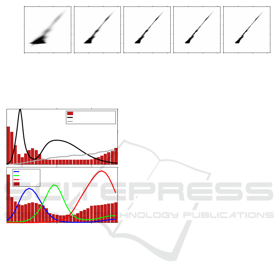
Figure 2: Checking the stability in the bad-SNR range of the monochrome camera: Response histograms on filtered, dark-
subtracted (offset by 30) input images after applying Gaussian filters of increasing size. As one can see, negative values after
dark-subtraction need to be taken into account since a clipping would bias the result largely. The camera’s output in this range
is statistically stable despite the fact that the output of the single pixels is shot-noise limited. Due to the stability, data in this
pixel value range can be used as an input for our method.
10
0
10
1
10
2
exposure time [s]
[relative]
exposure time (s)
LED normalized intensity
CCD quantum efficiency
10
1
10
2
10
3
filter size (pixels)
450 550 650
[relative]
blue sens.
green sens.
red sens.
filter sizes
Figure 3: Calibration of the measurement setup. The bar
plots show the resulting exposure times (top) and filter sizes
(bottom).
shown in Figure 3.
For the spectral camera, much more care has to be
taken since here measurements with a very low SNR
will be used. Therefore, the calibration of the cam-
era must also hold for low pixels values - a range that
is typically excluded using weighting functions. We,
however, want to use this range as well because we
use largely underexposed band-filtered images as in-
put data. We therefore require a calibration which is
exact for the low pixel values, too.
The first step is to obtain exact knowledge about
the camera’s dark current in all pixels. For this we
took 200 photographs with closed shutter and re-
peated this process for different exposure times. The
average over the dark frames is computed with float-
ing point accuracy.
To recover the OECF in the low-pixel-value range,
we propose to apply the Robertson algorithm to im-
ages modified by dark-subtraction, filtering and a re-
scaling to the full range of integers corresponding to
the camera’s bit depth. The filtering is done using a
Gaussian kernel as in the spectral recovery method.
As the original algorithm works on discrete inte-
ger pixel values, a mapping from the real-valued fil-
tered data has to be applied to obtain integers again.
As we take the images with short exposure times, the
filtered pixel values all lie in the lower range of the en-
tire interval of valid pixel values. We therefore stretch
this small interval to the full length and round these
new values to their respective nearest integers. These
new integer values can then directly be used in the
standard Robertson algorithm.
To show the effect of filtering on response recov-
ery, we computed response histograms for an expo-
sure series having extremely low pixel values. Fig-
ure 2 shows the histograms for different filter sizes.
The response of the camera is stable under filtering
even for pixel values with an SNR of 1 or smaller.
Notice, that the dark-current-noise of the camera is
Gaussian with standard deviation 3. The discrete na-
ture of the photo and electron shot-noise completely
cancels out when multiple pixels are combined by fil-
tering. The spectral calibration of our system means
straightforwardly taking images of a white diffuse ref-
erence surface under the known LED illumination and
dividing the response by the LED spectrum. The re-
sulting sensitivity for each wavelength band can be
taken from Figure 3. Finally, we checked the com-
plete calibration of both types of cameras by a cross-
validation experiment. This is done by simulating
the RGB response to an X-Rite colorchecker passport
from a spectral image taken with the spectral cam-
era system. This way all calibration results are com-
bined. The simulated RGB response matches the real
response extremely well which is shown in Figure 4.
GRAPP 2017 - International Conference on Computer Graphics Theory and Applications
154

(a) Real RGB data (b) Simulated RGB data (c) Difference ×10
Figure 4: Cross validation of the spectral calibration: (a)
real response of RGB cameras to color checker fields, (b)
simulation of responses by applying the RGB filter matrix
C to a spectral image captured using the spectral camera
system, (c) 10× scaled difference image showing that our
calibration used to generate the image in (b) is very exact.
5 EVALUATION
Prerequisites. For the evaluation of our method, we
used four challenging datasets: a red fabric made
of four different yarns, a collection of colorful Lego
bricks, a hand-made color checker with diffuse and
specular fields and a wallpaper having an embossed
structure. For all of these samples, complete spectral
ground truth data is available that was captured with
a gonioreflectometer setup (Rump et al., 2010).
Simulated Data. To evaluate the reconstruction
quality achievable by our method, we first performed
simulations based on spectral ground truth data. This
is extremely helpful because a pixel-wise comparison
between reference and reconstruction can be made.
This is not easily possible when using real data since
the geometries and resolutions of the setup used for
the ground truth measurements and the setup de-
scribed in Section 4 are quite different. Furthermore,
a basic understanding about the method and its prop-
erties can be gained without having too much bias by
real-world data.
To have a scenario as realistic as possible, we per-
formed a detailed simulation of the capture process.
For the image capture in the CCD cameras the cali-
bration results from Section 4 are used. The below
equation describes how a pixel value I is generated
from an incident irradiance x and exposure time t by
means of the camera mapping g : R → N:
I = g(x,t) :=
f
−1
(x ·t · Q
λ
) + ∆
ADC
+ N
σ
(5)
The I still has to be clamped to the valid range of
pixel values, in the case of our cameras to 10 bit un-
signed integers. Q
λ
denotes the combined quantum
efficiency of optical system and sensor at wavelength
λ and f
−1
is the OECF i.e. the inverse of the response
function. ∆
ADC
is the ADC offset of the camera and
N
σ
a random value drawn from a normal distribu-
tion with standard deviation σ mimicking the various
noise sources inside of the capture process. It is a
simplifying assumption to model the effect of the dif-
ferent capturing noise sources as Gaussian noise N
σ
.
However, this simplification is to some extend justi-
fied by the varying nature of the different noise com-
ponents. The values for f , Q, ∆
ADC
and σ are taken
from the calibration described in Section 4. We there-
fore end up with a detailed simulation of our mea-
surement setup that helps us to evaluate the quality of
spectral reconstruction in dependence on the different
parameters.
Starting with a spectral reference image S
re f
and
the spectral power distribution L of the illumination,
we first simulate an exposure series for the RGB im-
ages by computing I
RGB
(p) = g(CS
re f
(p)diag(L),t
i
)
for all pixels p of the reference image S
re f
and
for different exposure times t
i
. The RGB-LDR im-
ages are recombined to form HDR images using
Robertson’s algorithm (Robertson et al., 2003). For
the spectral images, one single exposure per wave-
length band is simulated by computing I
spectral
(p) =
g(S
re f
(p)diag(L),t
λ
).
During our experiments, it turned out to be the
best solution to use 4 different exposures t
i
for the
RGB cameras. For the spectral camera, we calculated
the exposure time according to equation 2. That is,
we accept more noise in those spectral bands having
bad support from light source and quantum efficiency.
The size of the Gaussian filters in the reconstruction
has to be adjusted accordingly.
Our simulation helps to choose good values for the
capture and reconstruction parameters in beforehand.
In Figure 3, we show the exposure times t
λ
for the
spectral camera system and the filter sizes of the gaus-
sian filters in the reconstruction process. The standard
deviation σ for the Gaussians was then set to 1/5 of
the filter size.
Full Correspondences. In many simple use cases,
just one spectral image needs to be taken. In this
case, the input to the reconstruction algorithm is a
high quality RGB image and all the band-filtered im-
ages corresponding to the wavebands of the spectral
camera (in our case 32, ranging from 410 to 720nm
in 10nm steps). We used one image (texture) per ex-
ample material as reference image. After running our
new algorithm, the result S is compared to the refer-
ence image S
re f
.
Figure 5 shows that our method successfully re-
covers spectral images that are very close to the
ground truth. We selected representative spectra by
picking both points with low and high RMSE in the
color mapped (Green, 2011) error maps. The highest
errors for the wallpaper material can be found in spec-
tra (4 – 6). The deviations occur mostly in the very
Fast Capture of Spectral Image Series
155
ground truth
1
2
3
4
5
6
normalized RMSE
1
2
3
4
5
6
0.005
0.025
0.05
0.075
0.095
450 550 650
1
450 550 650
2
450 550 650
3
450 550 650
4
450 550 650
5
450 550 650
6
(a) Wallpaper
ground truth
1
2
3
4
5
6
normalized RMSE
1
2
3
4
5
6
0.005
0.025
0.05
0.075
0.095
450 550 650
1
450 550 650
2
450 550 650
3
450 550 650
4
450 550 650
5
450 550 650
6
(b) Lego
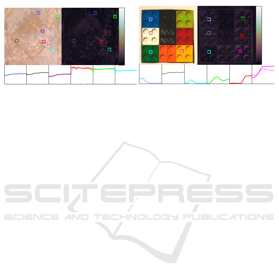
Figure 5: Normalized RMSE map of reconstructions of single images selected from two materials: shown respectively on the
left is the ground truth image (converted to RGB for display), whereas the right hand side shows an error map of the RMSE
of the reconstruction obtained from our simulated, artificially corrupted data. The pixel-wise RMSE is normalized by the
mean over all pixel intensities of the ground truth spectral image. Inset below are some representative ground truth (solid) and
reconstruction (dotted) spectra. Due to limited space, we omitted the reconstructed images as there is no noticable difference
in comparison with the ground truth when converted to RGB.
blue and red bands, which are the ones with the high-
est noise levels. For the vast majority of the pixels,
the two spectra are virtually indistinguishable. For
the Lego material, only spectrum (6) shows signifi-
cant deviations from the ground truth. This error oc-
curred in a highlight, which has a dramatically differ-
ent spectrum than the surrounding. We discuss these
errors in more detail in Section 6.
Sparsely Measured Spectral Bands. Reconstruct-
ing multiple images at once is the much more chal-
lenging case. Here, we aim at providing only
one noisy monochrome image per spectral band and
spread this information over several RGB images.
Even though there is no RGB image having complete
spectral information, the regularization helps to share
the information between the images. In this way, the
exposure time for the spectral camera system is kept
minimal and the spectral information can be acquired
simultaneously with the RGB data. Using this ap-
proach, spectral imaging can be accelerated to the
speed of RGB imaging and – in our use case – the
capture of spectral reflectance can be performed at the
speed of established RGB devices.
For our tests we capture 10 HDR RGB images
while acquiring all of the 32 noisy, band-filtered im-
ages, as we are able to achieve exactly these numbers
with our setup. Since the spectral camera is mounted
at 45
◦
elevation angle, we use only RGB images and
the corresponding noisy spectral data from this eleva-
tion. Additionally, we added 10 RGB images without
any spectral information and with different elevation
angles. This way, complete bi-angular reflectance can
be reconstructed using our method.
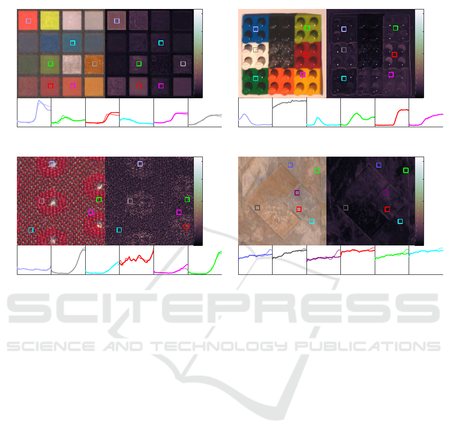
In Figure 6, error maps of the normalized RMSE
are shown. Figure 7 displays histograms that show
the cumulative behaviour over the entire experiments,
i.e. over all pixels of all the twenty images per mate-
rial. Both figures indicate that – just as in the single
image case – the errors are concentrated at low val-
ues, showing the high quality of the reconstruction.
The bin counts in the histograms of Figure 7 slightly
increase for the images captured at different elevation
angles than the one where the spectral camera was
placed. However, these increased errors are negligi-
ble considering the logarithmic scaling of the y-axis.
In the textures of Figures 5 and 6 there is no notica-
ble increase of the errors from the “known” images to
the “unknown” ones, which indicates that parallax ef-
fects have no large impact on the reconstruction qual-
ity. Therefore, high-quality spectral reflectance can
be captured at high speed using our method.
Real Data. To test our algorithm on real data, we
captured reference data for an X-Rite colorchecker
passport with our spectral camera system using a total
exposure time of 226212ms. Subsequently, we cap-
tured RGB and noisy band-filtered images with a total
exposure time of 7463ms and performed a reconstruc-
tion using our novel algorithm. Figure 8 shows a com-
parison between reference and reconstructed spectra
for some of the color fields. The figure shows that
our algorithm achieves nearly the same results as the
reference capture while requiring exposure times that
are about 1.5 orders of magnitude smaller. There
are again some more erroneous reconstructions at the
boundaries of the checker fields, which result from
gloss in these pixels and potentially a slight misalign-
GRAPP 2017 - International Conference on Computer Graphics Theory and Applications
156
Ω
i
= (30
°
, 150
°
), Ω
o
= (75
°
, 345
°
)
ground truth
1
2
3
4
5
6
normalized RMSE
1
2
3
4
5
6
0.01
0.05
0.1
0.15
0.19
450 550 650
1
450 550 650
2
450 550 650
3
450 550 650
4
450 550 650
5
450 550 650
6
(a) Color Checker
Ω
i
= (30
°
, 150
°
), Ω
o
= (60
°
, 36
°
)
ground truth
1
2
3
4
5
6
normalized RMSE
1
2
3
4
5
6
0.005
0.025
0.05
0.075
0.095
450 550 650
1
450 550 650
2
450 550 650
3
450 550 650
4
450 550 650
5
450 550 650
6
(b) Lego
Ω
i
= (0
°
, 0
°
), Ω
o
= (30
°
, 90
°
)
ground truth
1
2
3
4
5
6
normalized RMSE
1
2
3
4
5
6
0.01
0.05
0.1
0.15
0.19
450 550 650
1
450 550 650
2
450 550 650
3
450 550 650
4
450 550 650
5
450 550 650
6
(c) Red Fabric
Ω
i
= (30
°
, 150
°
), Ω
o
= (75
°
, 165
°
)
ground truth
1
2
3
4
5
6
normalized RMSE
1
2
3
4
5
6
0.01
0.05
0.1
0.15
0.19
450 550 650
1
450 550 650
2
450 550 650
3
450 550 650
4
450 550 650
5
450 550 650
6
(d) Wallpaper
Figure 6: Normalized RMSE maps for all of the four tested materials: We selected representative textures from elevations
(indicated respectively on the left as the first of the two angles of Ω
o
) different than the 45
◦
where we captured the band-
filtered images. Shown respectively on the left is the ground truth image (converted to RGB for display), whereas the right
hand side shows an error map of the RMSE of the reconstruction obtained from our simulated, artificially corrupted data. The
pixel-wise RMSE is normalized by the mean over all pixel intensities of the ground truth spectral image (notice the different
scaling of the colormap of the Lego material). Inset below are some representative ground truth (solid) and reconstruction
(dotted) spectra. Due to limited space, we omitted the reconstructed images as there is no noticable difference in comparison
with the ground truth when converted to RGB.
ment of the spectral bands and the RGB images.
6 LIMITATIONS
The reconstruction quality of our method depends
directly on how much the regularization biases the
result. Since it is assumed that similar RGB val-
ues have similar spectra, scenes containing two or
more metamers may pose problems. Especially for
reflectance capture, metamers may only occur for
certain azimuth angles, if anisotropic materials are
present. However, we consider the metamerism prob-
lem to be an extremely rare case and in our tests
this problem did not occur. Moreover, the problem
can be circumvented in many cases by adding spatial
proximity information to the appearance space pro-
jection to distinguish between metamers that are not
spatially adjacent. Another limitation is the occur-
rence of Fresnel reflections at certain elevation angles.
These reflections show both spectral and angular de-
pendence, as the refractive indices of material layers
vary with the wavelength. The assumption that spec-
tral data from only one elevation can be propagated
to the entire hemisphere can thus be violated by some
material classes. This limitation can, however, easily
be handled by addition of one or more spectral cam-
eras at different elevations.
Furthermore, the convergence speed of the spec-
tral recovery directly depends on the size of the Gaus-
sian filters used to get rid of the noise in the band-
filtered images. In effect, this limits the size of the fil-
ters and this way the acceptable noise level resulting
in a lower bound on the acceptable exposure times for
the spectral camera system. Of course, this problem
can be circumvented if a better optimization scheme
is used.
The last limitation arises from the proposed setup
only. Since we integrated only one spectral camera at
Fast Capture of Spectral Image Series
157
0 0.05 0.1 0.15 0.2 0.25
10
0
10
2
10
4
10
6
Color Checker - RMSE
with spectral corresp.
without spectral corresp.
0 0.1 0.2 0.3 0.4
10
0
10
2
10
4
10
6
Lego - RMSE
0 0.05 0.1 0.15
10
0
10
2
10
4
10
6
Red Fabric - RMSE
0 0.05 0.1 0.15 0.2 0.25 0.3
10
0
10
2
10
4
10
6
Wallpaper - RMSE
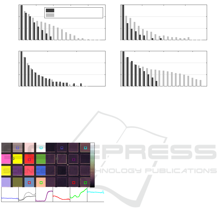
Figure 7: RMSE histograms for all of the four tested materials: For each of the four materials we compute a pixel-wise RMSE
over all the 32 channels. We separated the first ten images, which were measured at the 45
◦
elevation of the spectral camera,
from the remaining ten images where no spectral bands with pixel correspondences where acquired. In total, most of the
errors are close to zero with only a very small fraction of the pixels above an RMSE of ∼ 0.03 (notice the logarithmic scale of
the y-axis). As expected there is a noticable increase of the histogram counts for higher RMSEs for the images without direct
spectral correspondences. However, this increase occurs for a very small fraction of the pixels and is therefore perceptually
virtually unnoticeable, as can be seen in the other figures.
ground truth
1
2
3
4 5
6
normalized RMSE
1
2
3
4 5
6
0.01
0.05
0.1
0.15
0.19
450 550 650
1
450 550 650
2
450 550 650
3
450 550 650
4
450 550 650
5
450 550 650
6
Figure 8: Spectral reconstruction using real data: the left
part shows the RGB-converted ground truth data, the right
part the normalized RMSE between the reference and our
reconstruction. The reference data (solid plots) was ob-
tained using long exposure times and required a total ex-
posure time of 226212ms. The reconstruction by our al-
gorithm was based on shots with a total exposure time of
7463ms. The result indicates the robustness of our recon-
struction against high noise levels. Spectral imaging is ac-
celerated by about 1.5 orders of magnitude.
45
◦
elevation angle, materials showing dependence of
spectra on angle – like materials having interference
effects – cannot be reconstructed well. This, how-
ever, could be easily fixed by adding additional spec-
tral cameras.
7 CONCLUSIONS
In this paper, we presented a novel method for spec-
tral imaging, especially suited for the capture of mul-
tiple spectral images at once. Our method recon-
structs spectral images from high-quality RGB and
noisy band-filtered images using a novel variant of the
spectralization method. We have proven the stability
and quality of the method using both simulated and
real data. Due to the stability of our reconstruction
against noise in the band-filtered data, taking spec-
tral images can be vastly sped up. This way, spectral
imaging at the speed of RGB imaging is possible.
In general, our method is not limited to specialized
hardware like the RGB measurement device we used
to generate the data for our experiments. As long as a
reasonably good registration of RGB and spectral im-
ages is available, e.g. by using a beam splitter, our ap-
proach can be applied to reconstruct the spectral data
cube for one or multiple RGB images. Another po-
tential application would be the capturing of spectral
video. Here the only constraint is to capture enough
spectral band frames before the scene changes con-
siderably. The alignment between RGB and spectral
bands could be achieved with optical flow.
It should be noted that in the context of material
measurements there are certain constraints on the po-
sitioning of RGB and spectral cameras. To avoid par-
allax effects that arise as soon as materials are im-
aged that are not perfectly flat, the optical paths for
GRAPP 2017 - International Conference on Computer Graphics Theory and Applications
158

RGB and spectral cameras should match as closely
as possible. This can either be achieved by using a
beam splitter or by a similar setup like ours, where the
separation of the cameras matches exactly the angular
sampling of the material. Our approach should also be
applicable to image-based reflectance measurement
like the one developed by Hullin et al. (Hullin et al.,
2010). For the acquisition of HDR images, the au-
thors’ setup requires long measurement times with
exposures of up to 16s. Here, our method could pro-
vide a significant speed-up by decoupling spectral and
HDR acquisition using beam splitter optics, the exist-
ing combination of LCTF and monochrome camera,
and an additional monochrome or RGB camera to ac-
quire the HDR data.
In the future, it should be investigated whether the
applied principle is applicable using even more lev-
els of spectral resolution (e.g. monochrome, RGB,
and band-filtered), accepting different SNRs at the
different levels. Perhaps the presented method could
even help to get faster RGB imagery in certain use
cases since it can be straightforwardly applied to
monochrome and noisy RGB images. Other snapshot
spectral imaging techniques like CTIS could also be
used to provide the low-resolution spectral input data
as soon as the problem of spatially registering RGB
and spectral data is solved. Furthermore, it would be
helpful to have a better optimization scheme to allow
for a faster reconstruction.
ACKNOWLEDGEMENTS
This work was funded by the German Science Foun-
dation (DFG) under research grant KL 1142/7-1.
REFERENCES
Green, D. (2011). A colour scheme for the display
of astronomical intensity images. arXiv preprint
arXiv:1108.5083.
Hagen, N. and Kudenov, M. W. (2013). Review of snapshot
spectral imaging technologies. Optical Engineering,
52(9):090901–090901.
Hardeberg, J. Y., Schmitt, F., and Brettel, H. (2002). Multi-
spectral color image capture using a liquid crystal tun-
able filter. Optical Engineering, 40(10):2532–2548.
Hardeberg, J. Y., Schmitt, F., Brettel, H., Crettez, J.-P.,
and Maitre, H. (1999). Multispectral image acquisi-
tion and simulation of illuminant changes. In Colour
Imaging - Vision and Technology, pages 145–164. Wi-
ley.
Hullin, M. B., Hanika, J., Ajdin, B., Seidel, H.-P., Kautz, J.,
and Lensch, H. P. A. (2010). Acquisition and analy-
sis of bispectral bidirectional reflectance and reradia-
tion distribution functions. ACM Trans. Graph. (Proc.
SIGGRAPH 2010), 29(4):97:1–97:7.
Imai, F. H. and Berns, R. (1999). Spectral estimation using
trichromatic digital cameras. In Proceedings of the In-
ternational Symposium on Multispectral Imaging and
Color Reproduction, pages 42–49.
Imai, F. H. and Berns, R. S. (1998). High-resolution multi-
spectral image archives: A hybrid approach. Proc. of
the IS&T/SID Sixth Color Imaging Conference, pages
224–227.
Krishnan, D. and Fergus, R. (2009). Dark flash photogra-
phy. In ACM Transactions on Graphics, SIGGRAPH
2009 Conference Proceedings, volume 28.
Matsui, S., Okabe, T., Shimano, M., and Sato, Y. (2009).
Image enhancement of low-light scenes with near-
infrared flash images. In Asian Conference on Com-
puter Vision, pages 213–223. Springer.
Petschnigg, G., Szeliski, R., Agrawala, M., Cohen, M.,
Hoppe, H., and Toyama, K. (2004). Digital photogra-
phy with flash and no-flash image pairs. ACM trans-
actions on graphics (TOG), 23(3):664–672.
Robertson, M. A., Borman, S., and Stevenson, R. L. (2003).
Estimation-theoretic approach to dynamic range en-
hancement using multiple exposures. Journal of Elec-
tronic Imaging, 12(2):219–228.
Rump, M. and Klein, R. (2010). Spectralization: Recon-
structing spectra from sparse data. In SR ’10 Ren-
dering Techniques, pages 1347–1354, Saarbruecken,
Germany. Eurographics Association.
Rump, M., Sarlette, R., and Klein, R. (2010). Groundtruth
data for multispectral bidirectional texture functions.
In CGIV 2010, pages 326–330. Society for Imaging
Science and Technology.
Rump, M., Zinke, A., and Klein, R. (2011). Practical spec-
tral characterization of trichromatic cameras. ACM
Trans. Graph., 30(6).
Schwartz, C., Sarlette, R., Weinmann, M., Rump, M., and
Klein, R. (2014). Design and implementation of prac-
tical bidirectional texture function measurement de-
vices focusing on the developments at the university
of bonn. Sensors, 14(5).
Shrestha, R. and Hardeberg, J. Y. (2014). Evaluation and
comparison of multispectral imaging systems. In
Color and Imaging Conference, volume 2014, pages
107–112. Society for Imaging Science and Technol-
ogy.
Takeuchi, K., Tanaka, M., and Okutomi, M. (2013). Low-
light scene color imaging based on luminance es-
timation from near-infrared flash image. In Pro-
ceedings of IEEE International Workshop on Com-
putational Cameras and Displays (formerly PRO-
CAMS)(CCD/PROCAMS2013), pages 1–8.
Tsuchida, M., Arai, H., Nishiko, M., Sakaguchi, Y.,
Uchiyama, T., Yamaguchi, M., Haneishi, H., and
Ohyama, N. (2005). Development of BRDF and
BTF measurement and computer-aided design sys-
tems based on multispectral imaging. In Proc. AIC
Colour 05 – 10th congress of the international colour
association, pages 129–132.
Fast Capture of Spectral Image Series
159
