
Subspace Clustering and Visualization of Data Streams
Ibrahim Louhi
1,2
, Lydia Boudjeloud-Assala
1
and Thomas Tamisier
2
1
Laboratoire d’Informatique Th
´
eorique et Appliqu
´
ee, LITA-EA 3097, Universit
´
e de Lorraine, Ile du Saucly, Metz, France
2
e-Science Unit, Luxembourg Institute of Science and Technology, Belvaux, Luxembourg
Keywords:
Data Stream, Subspace Clustering, Visualization.
Abstract:
In this paper, we propose a visual subspace clustering approach for data streams, allowing the user to visually
track data stream behavior. Instead of detecting elements changes, the approach shows visually the variables
impact on the stream evolution, by visualizing the subspace clustering at different levels in real time. First we
apply a clustering on the variables set to obtain subspaces, each subspace consists of homogenous variables
subset. Then we cluster the elements within each subspace. The visualization helps to show the approach
originality and its usefulness in data streams processing.
1 INTRODUCTION
Data Mining aims to extract useful information from
raw data. Nowadays, technological advances allow
generating big amounts of data continuously, this data
is known as data streams. The processing of data
streams is very interesting problem, where classical
data mining techniques are not able to process this
kind of data. Streams processing is challenging be-
cause of many constraints that must be respected. A
data streams processing approach must imperatively
reflect the temporal aspect of data, follow the stream
evolution and generate results easily understandable
by the user. Clustering is one of data mining tech-
niques, it tries to put similar elements (according
to certain criteria) into a same group called cluster.
However, data can sometimes include hidden infor-
mation which are not visible on the original space of
variables. Within the techniques trying to discover
these information, subspace clustering looks for clus-
ters on all data subspaces. A subspace is composed
of a subset of variables. The challenge is to find rel-
evant subspaces offering more interesting results than
those on the original space of data. Subspace clus-
tering task is more complicated in data streams con-
text. In addition to the classical constraints of data
streams processing, subspaces must be evaluated over
the stream. Following the clusters evolution over time
and within different subspaces presents in itself a ma-
jor difficulty.
Complementarily to data mining, graphical repre-
sentations and visualization tools are used in order to
get a better understanding of the results. Visual anal-
ysis using graphics helps the user to better understand
the data characteristics detected by the data process-
ing. The challenge is to find an adequate representa-
tion that allows the user to use his cognitive abilities
and expertise to better analyze the results. Indeed,
by combining the processing efficiency of algorithms
and the perception abilities of humans, users can eas-
ily detect correlations in the results if they are well
represented graphically. Visualization in subspace
clustering context helps in addition to a better under-
standing of the results, to explore data at the level of
different subspaces. Many approaches were proposed
to apply subspace clustering on data streams, or to
visualize subspaces in static data. However, to our
knowledge, none allows to visualize in real time the
evolution of data stream and its subspaces.
In this paper we firstly present a brief state of
the art of some subspace clustering techniques of
static data, subspaces visualization tools, and sub-
space clustering of data streams. Then we present our
approach to apply a subspace clustering and visual-
ize results in real time at several levels. We discuss
the obtained results, and we illustrate the usefulness
of our approach and how to improve it.
2 STATE OF THE ART
Subspace clustering aims to identify subspaces of
variables, in order to find more interesting results.
Subspace clustering uses the original variables in-
stead of creating new ones (like in feature selection
Louhi I., Boudjeloud-Assala L. and Tamisier T.
Subspace Clustering and Visualization of Data Streams.
DOI: 10.5220/0006169702590265
In Proceedings of the 12th International Joint Conference on Computer Vision, Imaging and Computer Graphics Theory and Applications (VISIGRAPP 2017), pages 259-265
ISBN: 978-989-758-228-8
Copyright
c
2017 by SCITEPRESS – Science and Technology Publications, Lda. All rights reserved
259

techniques). As original variables are more signifi-
cant to the user unlike new created ones which are
hardly interpretable, subspace clustering allows a bet-
ter and more understandable representation of results
(Agrawal et al., 2005).
Subspace clustering tries to find all possible clus-
ters on all the subspaces, while identifying the better
subspace for each cluster. The challenge consists of
the big number of subspaces (possible combinations
of variables), hence the need of a research method
and an evaluation criteria to rank the subspaces. Sub-
spaces must be ranked for each cluster independently
of the other clusters. There are two types of subspace
clustering approaches depending on their technique
to find subspaces. Bottom-up algorithms find dense
regions into subspaces with low dimensionality and
combine them to form clusters. Top-down algorithms
find clusters in the original space of variables and then
they evaluate the subspaces of each cluster.
Bottom-up algorithms use the density downward
closure property to reduce the research space. They
create firstly a histogram of each dimension and
choose the one with a density above a threshold.
The density downward closure property means that if
there are dense units in k dimensions, there are dense
regions in all the projected units of the dimensions
k −1. Candidate subspaces on two dimensions can be
chosen using only the dimensions with dense units,
which reduces considerably the research space. And
so on the process is iterated until no more dense re-
gions remains. However, in this case, a cluster may
be separated by mistake in two smallest clusters. That
is way having good results strongly depends on grids
size and the density threshold.
CLIQUE (Agrawal et al., 1999) is one of the ear-
liest algorithms that tried to find clusters on data sub-
spaces. The algorithm combines a density-based and
a grid-based clustering techniques. It identifies the
dense subspaces, then it classifies them according to
their coverage (The coverage is a part of data cov-
ered by dense cells on the subspace). Subspaces with
the highest coverage are kept, then the algorithm finds
adjacent dense units on each selected subspace using
top-down research. Clusters are built by combining
these units using a greedy growth schema. The al-
gorithm starts by one arbitrary dense unit and builds
a maximal region in each dimension until the union
of all these regions covers all the cluster. CLIQUE
is able to find clusters with different shapes and rep-
resents them with an easily understandable way. EN-
CLUS (Cheng et al., 1999) is based on CLIQUE algo-
rithm, however, it does not measure directly the den-
sity or the coverage, but it measures the entropy. The
algorithm assumes that a subspace with clusters has
generally a lowest entropy than a subspace without
clusters. Three criteria define a subspace: coverage,
density and correlation, the entropy can be used to
measure all the three criteria. The entropy decreases
when the cells density increases, and under some con-
ditions, the entropy decreases when the coverage in-
creases. When interesting subspaces are found, clus-
ters can be identified using the same bottom-up ap-
proach as CLIQUE. MAFIA (Goil et al., 1999) is
an extension of CLIQUE which uses adaptative grids
based on the data distribution to improve the cluster-
ing efficiency and quality. Mafia creates an histogram
to determine the minimum number of cells in each di-
mension. The algorithm combines the adjacent cells
with a similar density to form bigger cells. Then it
uses the same process than CLIQUE to generate a list
of subspaces.
In data streams context, an adaptation of classical
subspace clustering techniques is necessary. DUC-
STREAM (Gao et al., 2005) is a grid-based algorithm
just like CLIQUE (Agrawal et al., 1999). In the same
way the data space is divided into units, and clus-
ters are obtained by the union of dense adjacent units.
DUCSTREAM performs an incremental update of the
units while detecting the changing units (from dense
to sparse for example). DUCSTREAM don’t need
to access to the previous data, it uses a resume of
the grid. HPSTREAM (Aggarwal et al., 2004) is an
adaptation of ClUSTREAM (Aggarwal et al., 2003)
which is a clustering algorithm for data streams. HP-
STREAM uses a micro-clustering to store a static re-
sume of the stream (clusters and their position in the
stream), and a macro-clustering which uses the re-
sume to provide the clustering results in each moment
of the stream. The clusters are obtained on subspaces,
and each subspace is continuously evaluated which
can change the obtained clusters structure. When a
new point arrives it is affected to the nearest clus-
ter on the same subspace or a new cluster is created.
A maximal number of cluster is fixed which requires
to delete the oldest ones. Contrary to HPSTREAM
which provides an approximatif result based on a re-
sume of the stream, INCPREDECON (Kriegel et al.,
2011) needs to access to the data (a limited access to
a subset of data only) to obtain better results. Based
on the new data at the instant T , the algorithm updates
the obtained clusters and their respective subspaces at
the instant T − 1.
In recent years, many visual approaches were pro-
posed for the subspace clustering. The use of humain
cognitive abilities can facilitate the understanding of
results. Despite the fact that machines have a big sta-
tistical and associative capacity, they can not equal the
cognitive perception of humans. Users can easily de-
IVAPP 2017 - International Conference on Information Visualization Theory and Applications
260

tect correlations and changes on data if the results are
well graphically represented (Keim, 2002). Visualiza-
tion plays an important role in the interaction between
users and the processing algorithm. Many visualiza-
tion techniques exist for data clustering on the entire
original space (Fayyad et al., 2002) (de Oliveira and
Levkowitz, 2003) (Keim et al., 2006) (Kovalerchuk
and Schwing, 2005) (Soukup and Davidson, 2002).
In this kind of clustering, clusters are visible only if
they are defined with all the variables set. The visu-
alization of clusters obtained within subspaces needs
adaptions of the classical techniques to represent hid-
den information to the user.
VISA (Assent et al., 2007) and MORPHEUS
(Muller et al., 2008) are visualization tools allowing
to obtain a significant overview of clusters on dif-
ferent subspaces, and to find the most relevant re-
sult. These tools display an overview of the sub-
space clustering using MDS (multidimensional scal-
ing) (Torgerson, 1958) to obtain 2D and 3D visualiza-
tions. 2D visualization is a static subspaces represen-
tation, however, the 3D visualization allows the user
to navigate on the subspace clustering results, to zoom
on the elements and to analyze subspaces features.
HEIDI MATRIX (Vadapalli and Karlapalem, 2009) is
a representation of subspaces using a matrix. The ma-
trix is based on k-nearest neighbors in each subspace.
Rows and Columns represent the elements, and each
cell (i, j) represents the number of subspaces where
the elements i and j are neighbors. Colors are used to
represent the combinations between subspaces. Fer-
dosi (Ferdosi et al., 2010) proposed an algorithm to
find subspaces within astronomical data and a visu-
alization tool to represent the results. The algorithm
identifies the candidate subspaces and uses density-
based measure to classify them. Subspaces are visu-
alized with different ways, a linear representation of
one dimension subspaces, a scatter plot visualization
for two dimensions subspaces and PCA projections
(Principal Component Analysis) (Pearson, 1901) for
more than two dimensions subspaces. CLUSTNAILS
(Tatu et al., 2012) is a tool allowing to analyze the
clusters using HeatNails, which are an extension of
heat maps. Rows represent dimensions and columns
the data. Each cell represents one element projected
on the corresponding dimension, and the elements are
regrouped by clusters. SUBVIS (Hund et al., 2016)
allows to visually analyze and explore the obtained
subspaces in three levels. The first level represents a
global overview of clusters on different subspaces and
their information (clusters and subspace size, vari-
ables distribution on different subspaces, and the sim-
ilarity between subspaces). In the second level, sub-
spaces can be detailed to show the distribution of each
cluster on the different subspaces. The elements can
be explored in the third level.
In our knowledge, there is no tool to find and vi-
sualize subspaces in data streams context. In this pa-
per, we propose our approach to automatically find
subspaces within data streams, and to visualize the re-
sult with the aim to find interesting information which
were not visible on the entire space of variables.
3 THE SUBSPACE CLUSTERING
In this work, we propose an approach to apply a vi-
sual subspace clustering on data streams. This ap-
proach is an extension of NNG Stream (Louhi et al.,
2016) which is neighborhood-based algorithm for
data streams processing (NNG: Nearest Neighbor-
hood Graph). Instead of processing each new element
individually just when it is generated, NNG-Stream
processes each group of new elements G
i
simultane-
ously. Groups size |G
i
| = n is fixed by the user accord-
ing to his expertise and preferences. Obtained clus-
ters on each new group are used to update the global
clusters of the stream according to a distance measure
(Euclidean distance) between the clusters medoids (a
medoid is the nearest element to the gravity center of
the cluster). Each cluster is visualized by a neigh-
borhood graph in order to reflect the processing al-
gorithm. In the following, we adapt NNG-Stream
for streams subspace clustering by allowing it to look
for clusters within the data subspaces (subset of vari-
ables), and to take into account the stream evolution
and the temporal aspect.
E = {e
1
, e
2
, ...} is the elements set of the stream
S, where the stream size |E| is unknown. D =
{d
1
, ..., d
m
} is the elements variables (dimensions)
set. When arrives the first group of elements
G
1
= {e
1.1
, ..., e
1.n
} represented by D, we apply a
neighborhood-based clustering algorithm on the vari-
ables set D. We measure the distance between each
pair of variables, two variables are neighbors if their
distance is smaller than a threshold. Each neighbors
group represents a cluster, and each cluster represents
a data subspace. Then for each obtained subspace, we
apply the neighborhood-based clustering on the ele-
ments considering only the subspace variables.
When arrives the next group G
2
= {e
2.1
, ..., e
2.n
},
we apply again the neighborhood-based clustering on
the variables set D. Two cases must be handled, either
we have the same subspaces than the first group (the
same clusters of variables), or the subspaces are dif-
ferent. If subspaces are the same, we process the ele-
ments of this second group G
2
in each subspace in the
same way as for the previous group G
1
and indepen-
Subspace Clustering and Visualization of Data Streams
261
dently of the previous results. Then the new clusters
are used to update the previous clusters. For each sub-
space, we measure the distance between the medoids
of the new and the previous clusters (the Euclidean
distance). If two medoids are close according to the
distance measure, we connect their respective clus-
ters. In the case where a new cluster is not close to
any of the previous clusters, it is added as a new clus-
ter in the stream. And so on, while subspaces are not
changing, we continue processing the stream group
by group and to update the previous clusters.
If when the new group arrives we have different
subspaces, we consider that the stream changed. Ob-
taining new subspaces means that there is a significant
change in the variables values. It also means that we
can not update the previous cluster anymore because
they are defined on different subspaces. This case rep-
resents the end of the first window, we keep a resume
of the window with the number and the variables of
each subspace as well as the number of clusters ob-
tained on each subspace. A window represents a part
of the stream T
i
→ T
j
with the same subspaces (T
i
is
the moment when the group G
i
is processed).
We process the groups elements of the second
window in the same way as the first one. Each time
that the subspaces change, it represents the end of the
current window, and at the end of each window we
keep a resume of the current subspaces and clusters.
The resume allows to track the changes of the stream.
The following algorithm details our approach.
Algorithm 1: Subspace Clustering.
Require: E = {e
1
, e
2
, ...} ; D = {d
1
, d
2
, ..., d
m
};
Ensure: Clusters defined on subspaces.
BEGIN
Wait for the first group G
1
= {e
1.1
, e
1.2
, ..., e
1.n
}.
Apply a clustering on D.
Clusters of D represent the subspaces SE
1
.
For each subspace, cluster the elements.
Wait for the second group G
2
= {e
2.1
, e
2.2
, ..., e
2.n
}.
Apply a clustering on D.
Clusters of D represent the subspaces SE
2
.
if SE
1
= SE
2
then
For each subspace, cluster the elements
Update the previous clusters
Iterate the algorithm on the next group
else
Close the window
Keep a resume of subspaces and clusters
Iterate the algorithm on the next window
end if
END.
4 VISUALIZATION, RESULTS
AND DISCUSSIONS
The aim of our approach is to apply a subspace clus-
tering on a data stream and to visualize the results on
different levels. In this section, we present an exam-
ple of a data stream processed by our approach and
the obtained visualizations. We use KDD99 data set
(Lichman, 2013) which is composed of 41 variables.
KDD99 is a networks firewall data, which includes a
wide variety of intrusions simulated in a military net-
work environment. The data is available as a text file
where each line represent a connection between two
IP adresses. The 41 variables describe the connec-
tions details.
Our interface includes several levels, a global
overview of the stream (figure 1), a subspaces visual-
ization (figures 2 and 3), a global overview of the ob-
tained clusters on each subspace (figures 4 to 8) and a
detailed visualization of the clusters on each subspace
(figure 6).
For the global overviews we use a visualization
inspired from the themerivers (Havre et al., 2002) to
represent the results. The x-axis of the themerivers
represents time (T
i
is the moment when the group G
i
is processed), and the y-axis represents the scale of
the rivers.
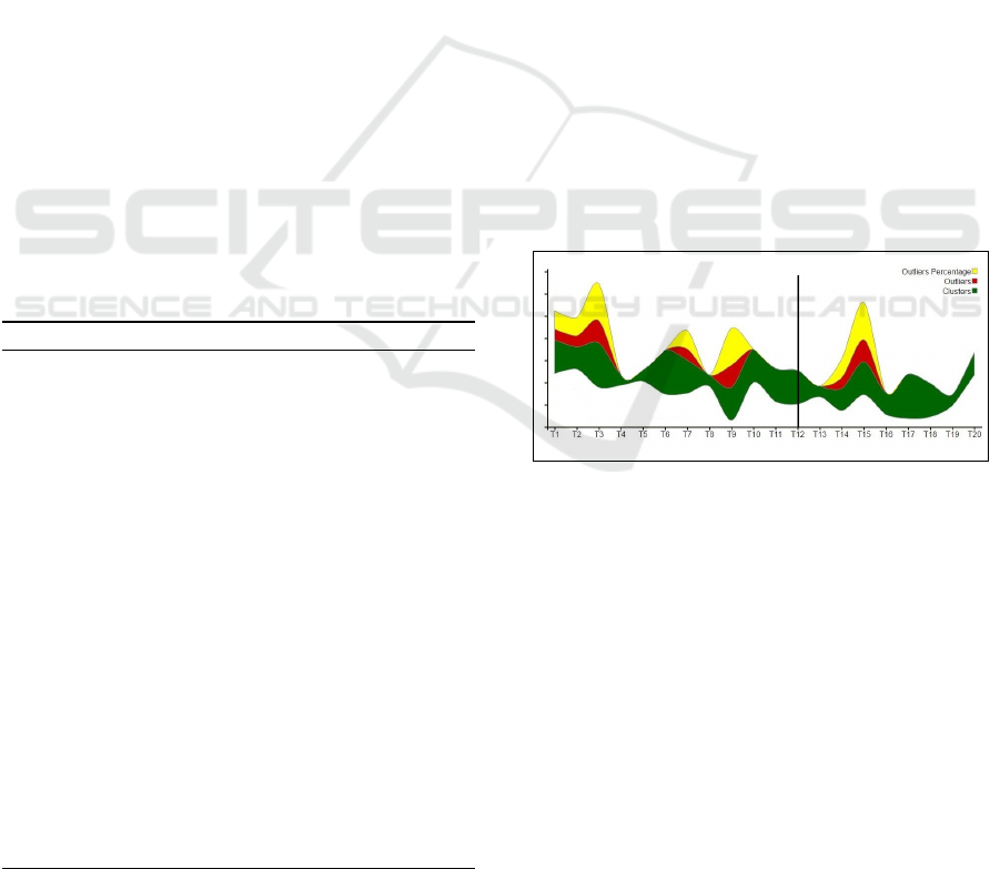
Figure 1: Global overview of data stream.
The figure 1 shows a part of the data stream rep-
resented by a themeriver. As we want to have a de-
scription of the clustering results obtained by NNG-
Stream (Louhi et al., 2016) on the entire original vari-
ables space, the rivers of the themeriver represent the
clusters number, the outliers number and the outliers
percentage according to the elements number, at each
instant T
i
(the outliers percentage is normalized ac-
cording to the clusters and outliers numbers). An out-
lier is an observation that deviates so much from other
observations as to arouse suspicion that it was gener-
ated by a different mechanism (Hawkins, 1980). We
choose to represent only these information on order to
have a simple visualization with a few details, allow-
ing the user to follow the stream evolution without a
big cognitive effort.
IVAPP 2017 - International Conference on Information Visualization Theory and Applications
262

Subspace clustering is applied in the same time as
NNG-Stream. At the end of each window (when the
subspaces change), a vertical line is displayed on the
themeriver (in our example, it is happening at the in-
stant T
12
). As it is explained in the previous section,
it means that the stream part from T
1
to T
12
has the
same subspaces. New subspaces are found after T
12
.
Our subspace clustering approach applies a cluster-
ing on the variables set in order to identify the sub-
spaces. Subspaces can be visualized (figures 2 and 3)
in the same time as the stream global overview. Each
point represents a variable and each cluster represents
a subspace.
Figure 2: Subspaces
between T1 and T12.
Figure 3: Subspaces
between T13 and T20.
Then a clustering is applied on the elements of
each subspace. Themerivers describing an overview
of the stream on each subspace can be obtained (fig-
ures 4, 5, 7 and 8).
Figure 4: The stream first window on the first subspace.
Figure 5: The stream first window on the second subspace.
On figures 4 and 5 themerivers represent a de-
scription of the clustering on the first window (T
1
to
T
12
) on the two subspaces separately. By comparing
these results with those of the clustering on the origi-
nal space, we note that on the first subspace (figure 4)
there are outliers in the same instants as in the global
clustering (T
3
and T
9
), and that outliers disappeared
at two instants (T
1
and T
6
). On the second subspace
(figure 5), we detect outliers at the same moment as
in the original space (T
1
, T
3
, T
6
and T
9
).
From the themerivers, the user can display de-
tailed clusters obtained at any instant T
i
. The figure 6
represents as an example the obtained clusters at T
15
on the first subspace where there is an appearance of
outliers. Clusters are represented with neighborhood
graphs in order to reflect the processing algorithm.
Figure 6: Clusters at T15on the first subspace.
This clusters visualization allows to compare de-
tected outliers on the original space with those de-
tected on the subspaces. At T
3
and T
9
two outliers are
detected on the original space at both instants, only
one of the outliers is detected on the first subspace
at both instants. On the second subspace, two out-
liers are detected at T
3
and T
9
and they are the same
as those detected on the original space. At T
1
and T
6
the same outliers are detected on both the second sub-
space and the original space (one outliers at each in-
stant). We note also that the second subspace is close
enough to the original subspace, the themeriver of the
second subspace is very similar to the themeriver od
the original space of variables.
Figures 7 and 8 represent the second window of
the data stream (after T
12
) on both subspaces.
Figure 7: The stream second window on the first subspace.
A comparison with the results obtained on the
original space shows that on the first subspace (fig-
ure 7) there are outliers at the same moment as on
the original space (T
15
) and a new outlier appeared
at T
18
. On the second subspace (figure 8), the out-
Subspace Clustering and Visualization of Data Streams
263
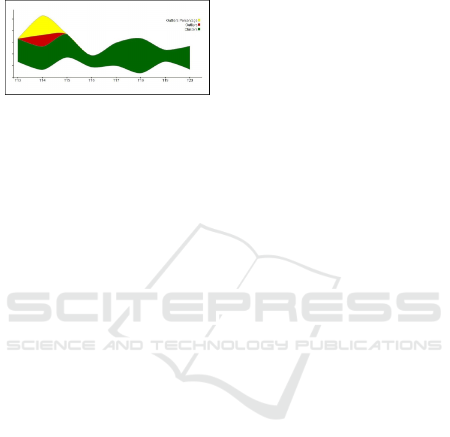
Figure 8: The stream second window on the second sub-
space.
liers disappeared at T
15
and new ones appeared at T
14
.
Clusters visualization with neighborhood graphs al-
lowed to compare the detected outliers. At T
14
the
same outlier is detected on both the original space and
the second subspace. At T
15
only one of the outliers
is detected on the first subspace.
Based on these visualizations (figures from 1 to 8)
we can clearly understand the interest of our approach
of subspace clustering for data streams. Applying a
clustering on the variables allows to group those with
the same influence on the data into the same cluster.
It was visible when we detected the same outliers on
the subspaces as in the original space. We also found
a subspace on which the stream has the same behav-
ior as on the original space (figure 5). We can easily
imagine the interest of representing the stream with
one subspace when we deal with high dimensional
data, allowing the optimization of the processing by
ignoring the irrelevant variables. We also detected
new outliers on subspaces while they don’t appear on
the original space. Which means that we discover in-
formation that were not visible on the original space.
The originality of the approach in addition to the
visualization of subspaces and their clusters in real
time over the stream evolution, is detecting the change
on the stream, not based on the elements behavior,
but by following the influence of variables on the ele-
ments. Change detection is generally done by statisti-
cal tests to follow the stream evolution. Our approach
follow the stream behavior under a completely differ-
ent point of view.
5 CONCLUSIONS
In this paper, we proposed a new visual approach to
apply a subspace clustering on data streams. In or-
der to find clusters on data subspaces, we apply a
clustering on the variables of the first group of ele-
ments. Clusters of variables represent subspaces, and
for each subspace, we apply a clustering on the ele-
ments. For the next group of elements, if we find the
same subspaces as the previous group, we process the
elements in the same way as the first group elements.
The new clusters are used to update the previous ones.
If new subspaces are founded, it represents the begin-
ning of a new window on the stream. The new win-
dow will be processed in the same way as the previous
one. At the end of each window, a resume is kept in
order to track the stream evolution.
Visualizing the subspace clustering steps allowed
to highlight the efficiency of this approach. We
successfully found subspaces representing the orig-
inal space of variables, a subspace on which the
stream had a different behavior (new information
were found), and the most important, we detected
changes on the stream under a new point of view. In-
stead of identifying the change by statistical tests, we
did it by focusing on the evolution of the impact of
variables on the stream.
For the future works, we intend to improve the ap-
proach by adding visualizations that follow the clus-
ters on the stream (which clusters merge and the split
clusters). We are also thinking about introducing
the concept drift, allowing for example to adapt the
groups size according to the prediction of stream evo-
lution. More evaluations will also be done, we will
use more data sets and evaluate the clusters and the
impact of the algorithm setting (groups size and dis-
tance threshold) on the results.
REFERENCES
Aggarwal, C. C., Han, J., Wang, J., and Yu, P. S. (2003).
A framework for clustering evolving data streams. In
Proceedings of the 29th international conference on
Very large data bases-Volume 29, pages 81–92. VLDB
Endowment.
Aggarwal, C. C., Han, J., Wang, J., and Yu, P. S. (2004).
A framework for projected clustering of high dimen-
sional data streams. In Proceedings of the Thirtieth
international conference on Very large data bases-
Volume 30, pages 852–863. VLDB Endowment.
Agrawal, R., Gehrke, J., Gunopulos, D., and Raghavan, P.
(2005). Automatic subspace clustering of high dimen-
sional data. Data Mining and Knowledge Discovery,
11(1):5–33.
Agrawal, R., Gehrke, J. E., Gunopulos, D., and Ragha-
van, P. (1999). Automatic subspace clustering of high
dimensional data for data mining applications. US
Patent 6,003,029.
Assent, I., Krieger, R., M
¨
uller, E., and Seidl, T. (2007).
Visa: visual subspace clustering analysis. ACM
SIGKDD Explorations Newsletter, 9(2):5–12.
Cheng, C.-H., Fu, A. W., and Zhang, Y. (1999). Entropy-
based subspace clustering for mining numerical data.
In Proceedings of the fifth ACM SIGKDD interna-
tional conference on Knowledge discovery and data
mining, pages 84–93. ACM.
IVAPP 2017 - International Conference on Information Visualization Theory and Applications
264

de Oliveira, M. F. and Levkowitz, H. (2003). From visual
data exploration to visual data mining: a survey. IEEE
Transactions on Visualization and Computer Graph-
ics, 9(3):378–394.
Fayyad, U. M., Wierse, A., and Grinstein, G. G. (2002). In-
formation visualization in data mining and knowledge
discovery. Morgan Kaufmann.
Ferdosi, B. J., Buddelmeijer, H., Trager, S., Wilkinson,
M. H., and Roerdink, J. B. (2010). Finding and
visualizing relevant subspaces for clustering high-
dimensional astronomical data using connected mor-
phological operators. In Visual Analytics Science and
Technology (VAST), 2010 IEEE Symposium on, pages
35–42. IEEE.
Gao, J., Li, J., Zhang, Z., and Tan, P.-N. (2005). An in-
cremental data stream clustering algorithm based on
dense units detection. In Pacific-Asia Conference on
Knowledge Discovery and Data Mining, pages 420–
425. Springer.
Goil, S., Nagesh, H., and Choudhary, A. (1999). Mafia: Ef-
ficient and scalable subspace clustering for very large
data sets. In Proceedings of the 5th ACM SIGKDD In-
ternational Conference on Knowledge Discovery and
Data Mining, pages 443–452. ACM.
Havre, S., Hetzler, E., Whitney, P., and Nowell, L. (2002).
Themeriver: Visualizing thematic changes in large
document collections. IEEE transactions on visual-
ization and computer graphics, 8(1):9–20.
Hawkins, D. M. (1980). Identification of outliers, vol-
ume 11. Springer.
Hund, M., B
¨
ohm, D., Sturm, W., Sedlmair, M., Schreck, T.,
Ullrich, T., Keim, D. A., Majnaric, L., and Holzinger,
A. (2016). Visual analytics for concept exploration in
subspaces of patient groups. Brain Informatics, pages
1–15.
Keim, D. A. (2002). Information visualization and visual
data mining. IEEE transactions on Visualization and
Computer Graphics, 8(1):1–8.
Keim, D. A., Mansmann, F., Schneidewind, J., and Ziegler,
H. (2006). Challenges in visual data analysis. In
Tenth International Conference on Information Visu-
alisation (IV’06), pages 9–16. IEEE.
Kovalerchuk, B. and Schwing, J. (2005). Visual and spa-
tial analysis: advances in data mining, reasoning, and
problem solving. Springer Science & Business Media.
Kriegel, H.-P., Kr
¨
oger, P., Ntoutsi, I., and Zimek, A. (2011).
Density based subspace clustering over dynamic data.
In International Conference on Scientific and Statisti-
cal Database Management, pages 387–404. Springer.
Lichman, M. (2013). Uci machine learning repository.
https://archive.ics.uci.edu/ml/datasets/KDD+Cup+19
99+Data. (consulted on: 11.12.2015).
Louhi, I., Boudjeloud-Assala, L., and Tamisier, T. (2016).
Incremental nearest neighborhood graph for data
stream clustering. In 2016 International Joint Con-
ference on Neural Networks, IJCNN 2016, Vancouver,
BC, Canada, July 24-29, 2016, pages 2468–2475.
Muller, E., Assent, I., Krieger, R., Jansen, T., and Seidl,
T. (2008). Morpheus: interactive exploration of sub-
space clustering. In Proceedings of the 14th ACM
SIGKDD international conference on Knowledge dis-
covery and data mining, pages 1089–1092. ACM.
Pearson, K. (1901). Liii. on lines and planes of closest fit to
systems of points in space. The London, Edinburgh,
and Dublin Philosophical Magazine and Journal of
Science, 2(11):559–572.
Soukup, T. and Davidson, I. (2002). Visual data mining:
Techniques and tools for data visualization and min-
ing. John Wiley & Sons.
Tatu, A., Zhang, L., Bertini, E., Schreck, T., Keim, D.,
Bremm, S., and Von Landesberger, T. (2012). Clust-
nails: Visual analysis of subspace clusters. Tsinghua
Science and Technology, 17(4):419–428.
Torgerson, W. S. (1958). Theory and methods of scaling.
Vadapalli, S. and Karlapalem, K. (2009). Heidi matrix:
nearest neighbor driven high dimensional data visu-
alization. In Proceedings of the ACM SIGKDD Work-
shop on Visual Analytics and Knowledge Discovery:
Integrating Automated Analysis with Interactive Ex-
ploration, pages 83–92. ACM.
Subspace Clustering and Visualization of Data Streams
265
