
Regularized Nonlinear Discriminant Analysis
An Approach to Robust Dimensionality Reduction for Data Visualization
Martin Becker
1,2,3
, Jens Lippel
1
and Andr
´
e Stuhlsatz
1
1
Faculty of Mechanical and Process Engineering, University of Applied Sciences D
¨
usseldorf, M
¨
unsterstr. 156, 40476,
D
¨
usseldorf, Germany
2
Faculty of Electrical Engineering and Information Technology, University of Applied Sciences D
¨
usseldorf, D
¨
usseldorf,
Germany
3
Faculty of Media, University of Applied Sciences D
¨
usseldorf, D
¨
usseldorf, Germany
Keywords:
High-dimensional Data, Dimensionality Reduction, Data Visualization, Discriminant Analysis, GerDA, Deep
Autoencoder, Deep Neural Networks, Regularization, Machine Learning.
Abstract:
We present a novel approach to dimensionality reduction for data visualization that is a combination of two
deep neural networks (DNNs) with different objectives. One is a nonlinear generalization of Fisher’s linear
discriminant analysis (LDA). It seeks to improve the class separability in the desired feature space, which is
a natural strategy to obtain well-clustered visualizations. The other DNN is a deep autoencoder. Here, an
encoding and a decoding DNN are optimized simultaneously with respect to the decodability of the features
obtained by encoding the data. The idea behind the combined DNN is to use the generalized discriminant
analysis as an encoding DNN and to equip it with a regularizing decoding DNN. Regarding data visualization,
a well-regularized DNN guarantees to learn sufficiently similar data visualizations for different sets of samples
that represent the data approximately equally good. Clearly, such a robustness against fluctuations in the
data is essential for real-world applications. We therefore designed two extensive experiments that involve
simulated fluctuations in the data. Our results show that the combined DNN is considerably more robust
than the generalized discriminant analysis alone. Moreover, we present reconstructions that reveal how the
visualizable features look like back in the original data space.
1 INTRODUCTION
Mapping high-dimensional data – usually containing
many redundant observations – onto 1, 2 or 3 features
that are more informative, often is a useful first step
in data analysis, as it allows to generate straightfor-
ward data visualizations such as histograms or scatter
plots. A fundamental problem arising in this context
is that there is no general answer to the question of
how one is supposed to choose or even design a map-
ping that yields these informative features. Finding a
suitable mapping typically requires prior knowledge
about the given data. At the same time, knowledge is
what we hope to be able to derive after mapping the
data onto informative features. Frequently, one might
know nothing or only very little about the given data.
In any case, one needs to be very careful not to mis-
take crude assumptions for knowledge, as this may
lead to a rather biased view on the data. So in sum-
mary, it appears as a closed loop “knowledge ⇒ map-
ping ⇒ informative features ⇒ knowledge”, where
each part ultimately depends on the given data and
the only safe entry point is true knowledge.
Deep neural networks (DNNs) have been proven
capable of tackling such problems. A DNN is a model
that covers an infinite number of mappings, which
is realized through millions of adjustable real-valued
network parameters. Rather than directly choosing a
particular DNN mapping, the network parameters are
gradually optimized (DNN learning) with respect to
a criterion that indicates whether or not a mapping of
a given dataset is informative. Two DNNs that have
been shown to be able to successfully learn useful
data visualizations are the Generalized Discriminant
Analysis (GerDA) and Deep AutoEncoders (DAEs)
as suggested by (Stuhlsatz et al., 2012) and (Hinton
and Salakhutdinov, 2006), respectively. A closer look
at these two DNNs reveals that the ideas of what the
term “informative” means can be very different.
GerDA is a nonlinear generalization of Fisher’s
Linear Discriminant Analysis (LDA) (Fisher, 1936)
116
Becker M., Lippel J. and Stuhlsatz A.
Regularized Nonlinear Discriminant Analysis - An Approach to Robust Dimensionality Reduction for Data Visualization.
DOI: 10.5220/0006167501160127
In Proceedings of the 12th International Joint Conference on Computer Vision, Imaging and Computer Graphics Theory and Applications (VISIGRAPP 2017), pages 116-127
ISBN: 978-989-758-228-8
Copyright
c
2017 by SCITEPRESS – Science and Technology Publications, Lda. All rights reserved
and thus considers discriminative features to be most
informative, which appears as a very natural strategy
to generate well-clustered visualizations of labeled
data sets. DAEs, on the other hand, seek to improve
an encoder/decoder mapping
f
DAE
:= f
dec
◦ f
enc
, (1)
where f
enc
is a dimensionality reducing encoder (the
desired feature mapping) and f
dec
is the associated
decoder. Practically, this is achieved by defining a
criterion that measures the dissimilarity between the
data and the reconstructions obtained by encoding and
subsequent decoding. DAEs can therefore be learned
without the use of class labels. Here, reconstructable
features are considered to be most informative.
The novel Regularized Nonlinear Discriminant
Analysis (ReNDA) proposed in this paper uses the
combined criterion
J
ReNDA
:= (1 − λ)J
GerDA
+ λ J
DAE
(λ ∈ [0|1]), (2)
where the two subcriteria J
GerDA
and J
DAE
are based
on GerDA and a DAE, respectively. As the name
suggests, we expect the associated ReNDA DNN to
be better regularized. Regularization is a well-known
technique to improve the generalization capability of
a DNN. Regarding dimensionality reduction for data
visualization, a good generalization performance is
indicated by a reliably reproducible 1D, 2D or 3D
feature mapping. In other words, a well-regularized
DNN guarantees to learn sufficiently similar feature
mappings for different sets of samples that represent
the data approximately equally good. Clearly, such a
robustness against fluctuations in the data is essential
for real-world applications.
Indeed, based on the belief that a feature mapping
learned by a DNN should be as complex as necessary
and as simple as possible, regularization of DNNs is
traditionally imposed in the form
J
effective
:= J
obj
+ λJ
reg
(λ ∈ [0|∞)), (3)
which looks very similar to the combined criterion
(2). Here, λ is a hyperparameter that is adjusted to
control the impact of a regularization term J
reg
on the
DNN’s true objective J
obj
. Well-known approaches
following (3) are weight decay (encouraging feature
mappings that are more nearly linear) and weight
pruning (elimination of network parameters that are
least needed) (cf. (Duda et al., 2000)). Both these
measures are intended to avoid the learning of overly
complex mappings. The advantage of (2) over these
two approaches is that both subcriteria are themselves
informative as regards the given data, whereas in most
cases, weight decay or pruning can only tell us what
we already know: The present DNN covers overly
complex feature mappings.
X
0
:= X
W
1
,b
b
b
1
X
1
W
2
,b
b
b
2
X
2
.
.
.
X
L−1
W
L
,b
b
b
L
X
L
:= Z
(W
L
)
tr
,b
b
b
L−1
X
L+1
.
.
.
X
2L−2
(W
2
)
tr
,b
b
b
1
X
2L−1
(W
1
)
tr
,b
b
b
2L
X
2L
:=
b
X
R
(0|1)
(0|1)
.
.
.
(0|1)
R
(0|1)
.
.
.
(0|1)
(0|1)
R
RBM
1
RBM
2
RBM
L
W,b
b
b
h
W,b
b
b
h
W,b
b
b
h
b
b
b
v
J
DAE
(decodability)
J
GerDA
(discriminability)
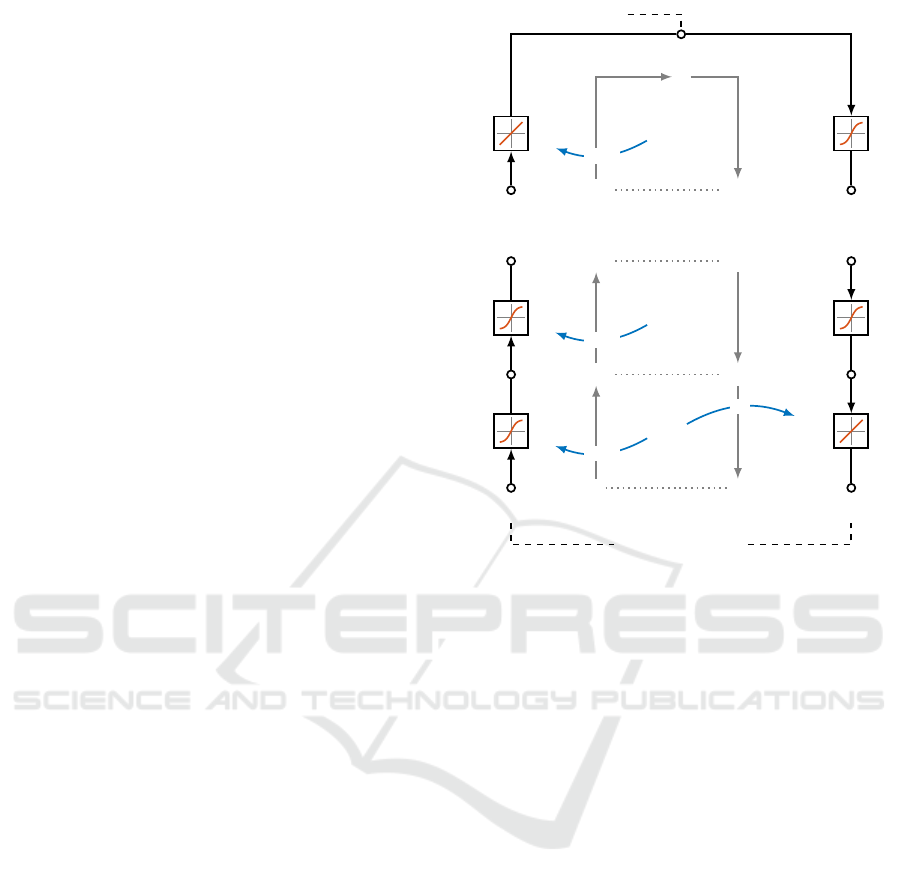
Figure 1: A data flow graph of the overall 2L-layered
ReNDA DNN. Each layer is depicted as a box containing
a symbolic plot of its activation function. The L layers on
the lefhand side form the encoding and the L layers on the
righthand side form the decoding DNN (cf. Sections 2.1 and
2.2). The inner “spaces flow graph” along with the RBMs
and the curved arrows concern the RBM-pretraining (cf.
Section 2.3). The GerDA criteron J
GerDA
is connected to
feature space node by a dashed line, where it takes direct
influence during fine-tuning (cf. Section 2.4). Accordingly,
J
DAE
takes direct influence at original space node and the
reconstruction space node.
2 ReNDA
As explained above, ReNDA is a combination of two
different DNNs, GerDA and a DAE. As a matter of
fact, both these DNNs learn feature mappings in a
very similar way, which is another reason why we
considered this particular combination: They both use
a Restricted Boltzmann Machine (RBM) pretraining
to determine good initial network parameters, which
are then used for subsequent gradient descent-based
fine-tuning. The big difference between them is that
a DAE involves an encoding ( f
enc
) and a decoding
( f
dec
) DNN, whereas GerDA involves an encoding
DNN only. So contrary to a DAE, GerDA is unable to
decode previously learned informative features.
The idea behind ReNDA is to equip GerDA with
a suitable decoding DNN and, additionally, introduce
it in such a way that it has a regularizing effect on
Regularized Nonlinear Discriminant Analysis - An Approach to Robust Dimensionality Reduction for Data Visualization
117

the encoding GerDA DNN. However, in this paper we
focus on presenting the developed ReNDA DNN as
a well-regularized and therefore robust approach to
data visualization. Figure 1 shows a detailed data flow
graph of the overall ReNDA DNN. In the following
four subsections we give a detailed explanation of all
elements depicted in this figure.
2.1 The Encoding DNN
Suppose that the columns of X := (x
x
x
1
,.. .,x
x
x
N
) ∈
R
d
X
×N
are d
X
-dimensional samples and that y
y
y :=
(y
1
,.. .,y
N
)
tr
∈ {1, ...,C}
N
is a vector of class labels
associated with these samples. ReNDA’s objective is
to find a DNN-based nonlinear encoding
X 7→ Z := f
enc
(X) ∈ R
d
Z
×N
(4)
with d
X
> d
Z
∈ {1,2,3} that is optimal in the sense
of an LDA for data visualization, i.e. that the features
Z = (z
z
z
1
,.. .,z
z
z
N
) ∈ R
d
Z
×N
are both well-clustered with
respect to y
y
y and visualizable. The layerwise encoding
shown on the lefthand side of Figure 1 is obtained by
setting X
0
:= X, d
0
:= d
X
, X
L
:= Z, d
L
:= d
Z
and
defining
X
`
:= f
`
(W
`
X
`−1
+ B
`
| {z }
=:A
`
(X
`−1
)
) ∈ R
d
`
×N
(5)
for ` ∈ {1, ... ,L} and intermediate dimensions
d
1
,.. .,d
L−1
∈ N. We refer to d
0
-d
1
-d
2
-·· ·-d
L
as
the DNN topology. Further, A
`
(X
`−1
) ∈ R
d
`
×N
is
the `th layer’s net activation matrix and it depends
on the layer’s adjustable network parameters: the
weight matrix W
`
∈ R
d
`
×d
`−1
and the bias matrix
B
`
:= (b
b
b
`
,.. .,b
b
b
`
) ∈ R
d
`
×N
. The function f
`
: R → R
is called the `th layer’s activation function and it is
applied entrywise, i.e.
x
`
k,n
= f
`
(a
`
k,n
(X
`−1
)) (6)
for the entries of X
`
. The encoding DNN’s activation
functions are set to f
`
:= sigm with sigm : R → (0|1)
given by
sigm(x) :=
1
1 + exp(−x)
(x ∈ R) (7)
for ` ∈ {1,...,L − 1} and to f
L
:= id with id : R → R
given by
id(x) := x (x ∈ R), (8)
respectively. In Figure 1 the activation functions are
depicted as symbolic plots.
Altogether
f
enc
= f
L
◦ A
L
◦ ··· ◦ f
2
◦ A
2
◦ f
1
◦ A
1
| {z }
layerwise forward propagation
(9)
and optimizing it with respect to J
GerDA
(cf. Section
2.4.1) corresponds to the originally proposed GerDA
fine-tuning (Stuhlsatz et al., 2012). The dashed link
between J
GerDA
and the Z node of the data flow graph
shown in Figure 1 is a reminder that Z is the GerDA
feature space. With the decoding DNN presented in
the next section, Z will become the feature space of
the overall ReNDA DNN.
2.2 The Decoding DNN
As can be seen on the righthand side of Figure 1, the
adjustable network parameters of ReNDA’s encoding
DNN are reused for decoding
Z 7→
b
X := f
dec
(Z) ∈ R
d
b
X
×N
(10)
with d
b
X
:= d
X
. The final biases b
b
b
2L
∈ R
d
2L
represent
the only additional network parameters of ReNDA
compared to GerDA. We summarize by
θ
θ
θ := (W
1
,b
b
b
1
,.. .,W
L
,b
b
b
L
|
{z }
network parameters of
the encoding DNN
,b
b
b
2L
) (11)
the network parameters of the ReNDA DNN. One of
the main reasons for this kind of parameter sharing is
that it connects f
enc
and f
dec
at a much deeper level
than (2) alone. Observe that J
GerDA
and J
DAE
only
take direct influence at three points of the ReNDA
DNN. We stated in the introduction that a DNN has
typically millions of adjustable real-valued network
parameters. So between the two criteria there also lie
millions of degrees of freedom. Here, it is very likely
that f
dec
compensates for a rather poor f
enc
or vice
versa. In this case, the two mappings would not be
working together. Considering this, we can specify
what we mean by a connection of f
enc
and f
dec
at a
deeper level: The parameter sharing ensures that the
two DNNs work on the very same model. It makes
the decoding DNN a supportive and complementing
coworker that helps to tackle the existing task rather
than causing new, independent problems.
We conclude this section with the mathematical
formulation of the weight sharing as it is depicted in
Figure 1. To provide a better overview, we arranged
the layers as horizontally aligned encoder/decoder
pairs that share a single weight matrix: Layer ` = 2L
uses the transposed weight matrix (W
1
)
tr
of the first
layer. Layer ` = 2L − 1 uses the transposed weight
matrix (W
2
)
tr
of the second layer. So in general,
W
`
=
W
2L−`+1
tr
(12)
and d
`
= d
2L−`
for ` ∈ {L + 1, ... ,2L}, which implies
d
2L
= d
0
= d
X
= d
b
X
. Note that the decoding DNN
has the inverse encoding DNN topology d
L
-.. .-d
0
.
IVAPP 2017 - International Conference on Information Visualization Theory and Applications
118

We can therefore still write d
0
-.. .-d
L
for the DNN
topology of the overall ReNDA DNN. In the case of
the biases, we see that
b
b
b
`
= b
b
b
2L−`
(13)
for ` ∈ {L + 1,.. .,2L − 1}. Observe that (13) does
not include the additional final decoder bias vector
b
b
b
2L
because there is no d
0
-dimensional encoder bias
vector that can be reused at this point. The symbolic
activation function plots indicate that
f
`
=
(
sigm L + 1 ≤ ` ≤ 2L − 1
id ` = 2L .
(14)
Finally, we have that
f
dec
= f
2L
◦ A
2L
◦ ··· ◦ f
L+1
◦ A
L+1
(15)
with A
2L
,.. .,A
L+1
according to (5). It is
X 7→
b
X = ( f
dec
◦ f
enc
)(X) = f
DAE
(X) (16)
and optimizing f
DAE
with respect to J
DAE
(cf. Section
2.4.2) corresponds to the originally proposed DAE
fine-tuning (Hinton and Salakhutdinov, 2006). Here,
J
DAE
measures the dissimilarity between the samples
X and its reconstructions
b
X. In the data flow graph
shown in Figure 1 this is symbolized by a dashed line
from the X node to J
DAE
to the
b
X node.
2.3 RBM-Pretraining
As mentioned earlier, both GerDA and DAEs use an
RBM-pretraining in order to determine good initial
network parameters. In this context, “good” means
that a subsequent gradient descent-based fine-tuning
has a better chance to approach a globally optimal
mapping. Randomly picking a set of initial network
parameters, on the other hand, almost certainly leads
to mappings that are rather poor and only locally op-
timal (Erhan et al., 2010). As an in-depth explanation
of the RBM-pretraining would go beyond the scope
of this paper, we will only give a brief description of
the according RBM elements shown in the data flow
graph (cf. Figure 1).
Here, we see that there exists an RBM for each
horizontally aligned encoder/decoder layer pair. Each
RBM
`
for ` ∈ {1, ... ,L} is equipped with a weight
matrix W ∈ R
d
`−1
×d
`
, a vector b
b
b
v
∈ R
d
`−1
of visible
biases and a vector b
b
b
h
∈ R
d
`
of hidden biases. Once
pretrained the weights and biases are passed to the
DNN as indicated by the curved arrows. This is the
exact same way in which the network parameters of
the original GerDA DNN are initialized. Again, the
only exception is the final bias vector b
b
b
2L
. Here, the
bias b
b
b
v
of RBM
1
is used. The initialization of the
remaining network parameters of the decoding DNN
follows directly from the parameter sharing (12) and
(13) introduced in Section 2.2.
2.4 Fine-tuning
Now, for the gradient descent-based fine-tuning we
need to specify the two criteria J
GerDA
and J
DAE
. It
turned out that when combining the two criteria one
has to pay attention to their orders of magnitude. We
determined the following normalized criteria to be
best working.
2.4.1 Normalized GerDA Criterion
Before we present our normalization of the GerDA
criterion, we shall review the original criterion
Q
δ
z
:= trace
(S
δ
T
)
−1
S
δ
B
(17)
as suggested by (Stuhlsatz et al., 2012). Here, it has
been shown that maximizing Q
δ
z
yields well-clustered,
visualizable features. The two matrices appearing in
(21) are: The weighted total scatter matrix
S
δ
T
:= S
W
+ S
δ
B
(18)
with the common (unweighted) within-class scatter
matrix S
W
:= (1/N)
∑
C
i=1
N
i
Σ
Σ
Σ
i
of the class covariance
matrices Σ
Σ
Σ
i
:= (1/N
i
)
∑
n: y
n
=i
(z
z
z
n
−m
m
m
i
)(z
z
z
n
−m
m
m
i
)
tr
with
the class sizes N
i
:=
∑
n: y
n
=i
1 and the class means
m
m
m
i
:= (1/N
i
)
∑
n: y
n
=i
z
z
z
n
. The weighted between-class
scatter matrix
S
δ
B
:=
C
∑
i, j=1
N
i
N
j
2N
2
· δ
i j
· (m
m
m
i
− m
m
m
j
)(m
m
m
i
− m
m
m
j
)
tr
(19)
with the global symmetric weighting
δ
i j
:=
(
1/km
m
m
i
− m
m
m
j
k
2
i 6= j
0 i = j.
(20)
Clearly, δ
i j
is inversely proportional to the distance
between the class means m
m
m
i
and m
m
m
j
. The idea behind
this is to make GerDA focus on classes i and j that are
close together or even overlapping, rather than ones
that are already far apart from each other.
For ReNDA, we modified Q
δ
z
as follows:
J
GerDA
:= 1 −
Q
δ
z
d
Z
∈ (0|1) (21)
The division through d
Z
is the actual normalization
(cf. Appendix A). Subtracting this result from one
makes J
GerDA
a criterion that has to be minimized,
which is a necessary in order to be able to perform
gradient descent for optimization. See Appendix B
for the partial derivatives of J
GerDA
.
Regularized Nonlinear Discriminant Analysis - An Approach to Robust Dimensionality Reduction for Data Visualization
119

2.4.2 Normalized DAE Criterion
During our first experiments, we used the classical
mean squared error
MSE :=
1
N
k
b
X − Xk
2
F
∈ [0|∞) (22)
with Frobenius norm
kUk
F
:=
s
m
∑
i=1
n
∑
j=1
|u
i, j
|
2
(U ∈ R
m×n
) (23)
as the DAE criterion. Here, the problem is that the
MSE is typically considerably greater than Q
δ
z
. Note
that (21) implies Q
δ
z
∈ (0|d
Z
). So in the context of
dimensionality reduction for data visualization where
d
Z
∈ {1,2,3} this difference in order of magnitude
is especially large. We therefore modified the DAE
criterion in the following way:
J
DAE
:=
MSE/d
X
1 + MSE /d
X
∈ [0|1) (24)
The division through d
X
was arbitrarily introduced.
Together with N it kind of prenormalizes k·k
2
F
before
the final normalization (·)/[1 + (·)]. It is part of our
future work to find whether or not there exists a better
denominator than d
X
, or even if there is a better way
of defining a normalized DAE criterion.
However, with J
GerDA
(cf. (21)) and J
DAE
having
the same bounded codomain, their combination is less
problematic. The partial derivatives of J
DAE
can be
found in Appendix C.
3 EXPERIMENTS
In the introduction we claimed that DNNs are able to
successfully learn dimensionality reducing mappings
that yield informative, visualizable features. For both
GerDA and DAEs this claim has been experimentally
proven: In (Stuhlsatz et al., 2012) and (Hinton and
Salakhutdinov, 2006), respectively, the widely used
MNIST database of handwritten digits (LeCun et al.,
1998) has been mapped into a 2D feature space. In an-
other example, GerDA has been used for an emotion
detection task. Here, 6552 acoustic features extracted
from speech recordings were reduced to 2D features
that allow to detect and visualize levels of valence and
arousal (Stuhlsatz et al., 2011).
In the following two sections, we experimentally
show that our expectations concerning ReNDA are
true, i.e. that ReNDA is also able to successfully learn
feature mappings for data visualization and that these
mappings are robust against fluctuations in the data,
which is due to improved regularization. In order to
-1 0 1
-1
0
1
-0.03 0 0.03
-0.03
0
0.03
Figure 2: A scatter plot of the artificial galaxy data set. The
plot on the righthand side shows a zoom of the center point
of the galaxy. Here, we see that the 3 classes are in fact
non-overlapping but very difficult to separate.
be able to see this improvement in regularization, we
ran all experiments for both ReNDA and GerDA and
compared their results.
Throughout all of the ReNDA experiments we set
λ = 0.5, mainly because it avoids prioritization of any
of the two criteria J
GerDA
and J
DAE
(cf. (2)), i.e. we
did not validate λ beforehand. It simply would have
been too computationally expensive.
3.1 Artificial Galaxy Data Set
To initially verify the expectations stated above, we
used the artificially generated galaxy-shaped data set
shown in Figure 2. Although it is already very easy
to visualize, DNN learning of optimal 1D features is
still challenging. The reason why we chose to use
an artificial rather than a real-world data set is that
most of the interesting real-world data sets are often
far too complex to obtain fast results. In the case of
the galaxy data set, the associated DNN parameters
are relatively fast to compute, which made it possible
to run very extensive experiments but with reasonable
computational effort.
3.1.1 Experimental Setup
The main goal of this experiment is to investigate the
influence of fluctuations in the data on the learned
ReNDA and GerDA visualizations. The results will
allow us to compare these two approaches as regards
their robustness.
We simulated fluctuations in the data by taking
10 distinct sets of samples from the galaxy data set,
which were then used for 10 ReNDA and 10 GerDA
runs. In detail, each of the 10 galaxy sets contains
1440 samples (480 per class) that were presented for
DNN learning, and additional 5118 samples (1706 per
class) that were used for validation. Further details on
how the samples are presented for DNN learning can
be found in the Appendix D.
For both ReNDA and GerDA we chose the DNN
IVAPP 2017 - International Conference on Information Visualization Theory and Applications
120
topology 2-20-10-1. This choice is based on the very
similar 3-40-20-10-1 DNN topology that (Stuhlsatz
et al., 2012) used to learn informative 1D features
from a 3-class artificial Swiss roll data set. Removing
the intermediate dimension 40 made DNN learning
more challenging while reducing the computational
effort. In other words, it yielded a less flexible DNN
mapping but with fewer parameters to optimize.
One very important aspect to consider is that the
algorithmic implementations of both ReNDA’s and
GerDA’s DNN learning, involve the use of a random
number stream. In this experiment we ensured that
this stream is the same for all 10 ReNDA and all 10
GerDA runs. The initial network parameters of the
RBM-pretraining are also based on this stream, which
implies that we do not include any potentially biased
parameter initializations. Moreover, any fluctuations
in both the ReNDA and the GerDA results are due to
the simulated fluctuations in the data only.
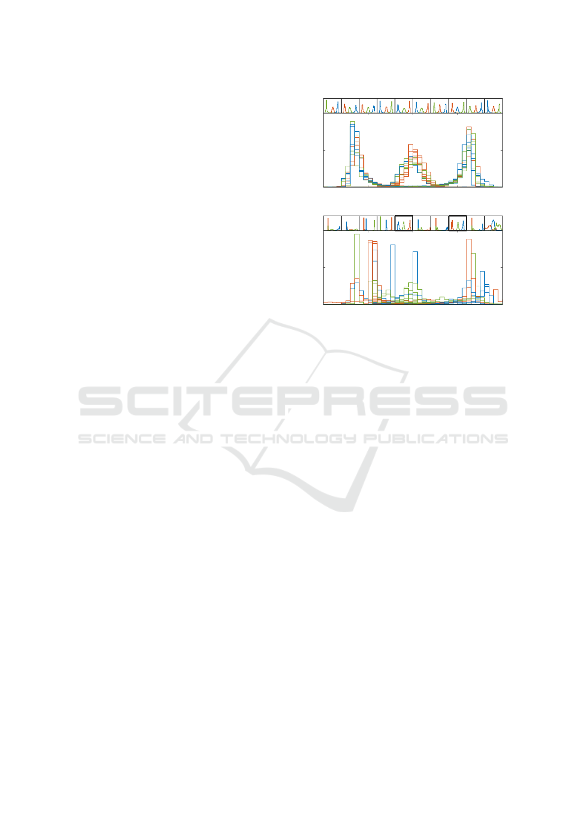
3.1.2 1D Visualization
We now compare the 1D mappings obtained from the
10 ReNDA and the 10 GerDA runs. To that end, we
use class-conditional histograms as a straightforward
method for 1D visualization. This is best explained
by directly discussing the results. In order to not get
things mixed up, we begin with the ReNDA results
shown in Figure 3(a) and discuss the GerDA results
(cf. Figure 3(b)) afterwards.
The top row of small plots in Figure 3(a) shows the
results of the individual ReNDA runs. Each of these
plots includes 3 distinct relative histograms that are
based on standardized 1D features associated with the
validation samples: One that considers the samples in
the red or asterisk (×+) class, a second for the green
or cross mark (×) class, and a third for the blue or
plus mark (+) class. The large plot in Figure 3(a)
represents an overlay of all small plots. Note that the
axis limits of all 11 plots are identical. Therefore, the
overlay plot indicates a high similarity between the
learned 1D mappings. Only the order of the 3 classes
changes throughout the different ReNDA runs, which
is due to the symmetry of the galaxy data set.
The corresponding GerDA histograms shown in
Figure 3(b) are organized in the very same way as in
Figure 3(a). Especially, two small histograms with the
same position in 3(b) and 3(a), respectively, are based
on the same 1440 samples for DNN learning and the
same 5118 samples for validation. However, here we
used differently scaled vertical axes depending on the
maximum bar height of each histogram. Observe that
only the two bold-framed histograms are similar to
the ReNDA histograms. Finally, the GerDA overlay
plot shows that the 1D mappings learned by GerDA
-2 -1 0 1 2
0
0.25
0.5
(a) ReNDA
-2 -1 0 1 2
0
0.5
1
(b) GerDA
Figure 3: A comparison of the 1D mappings learned by
ReNDA (a) and GerDA (b). The top row of small subplots
in (a) and (b), respectively, shows the histograms of the 1D
features associated with the validation samples of each of
the 10 galaxy data sets. The large plots represent overlays
of these 10 subplots.
are significantly less similar to each other than those
learned by ReNDA. In the case of GerDA, the three
classes are hardly to detect, whereas for ReNDA we
obtained 3 bump-shaped and easy to separate clusters.
The latter point, clearly shows that ReNDA is more
robust and thus better regularized than GerDA.
3.2 Handwritten Digits
Of course, the artificial galaxy data set used above is
neither high-dimensional nor an interesting example
from a practical point of view. We therefore decided
to run further experiments with the MNIST database
of handwritten digits (LeCun et al., 1998), a widely
used real-world and benchmark data set for the testing
of DNN learning approaches.
MNIST contains a large number of samples of
handwritten digits 0 to 9 stored as grayscale images
of 28×28 pixels. These samples are organized as two
subsets: a training set containing 60k samples and a
test set of 10k samples. Some examples taken from
the test set are show in Figure 6(a). With its 28 × 28
pixel images and variations in the handwriting it falls
into the category of big dimensionality data sets as
discussed in (Zhai et al., 2014). Nevertheless there are
no visible non-understood fluctuations present, which
is important for our experimental setup. As before,
Regularized Nonlinear Discriminant Analysis - An Approach to Robust Dimensionality Reduction for Data Visualization
121

we want to simulate the fluctuations in order to see
their effect on the feature mappings.
3.2.1 Experimental Setup
The setup of this experiment slightly differs from that
of the previous one. We again considered fluctuations
in data but also fluctuations in the random number
stream that both ReNDA and GerDA depend on (c.f.
Section 3.1.1). In practice, the latter fluctuations are
especially present when DNN learning is performed
on different computer architectures: Here, very much
simplified, different rounding procedures may lead
to significantly dissimilar mappings even if the same
samples are presented for DNN learning.
In this experiment we simulated these fluctuations
in the random number stream simply by generating 3
distinct random number streams with a single random
number generator. The fluctuations in the data were
simulated via 3 distinct random partitions of the 60k
training samples into 50k samples presented for DNN
learning, and 10k samples for validation. Finally, we
combined each of these 3 partitions with each of the
3 random number streams, which then allowed us to
realize 9 ReNDA and 9 GerDA runs. Further details
on how the samples are presented for DNN learning
can be found in Appendix D.
For both ReNDA and GerDA we chose the DNN
topology 784-1500-375-750-2 that was also used in
(Stuhlsatz et al., 2012) in order to be able to compare
our results in a meaningful way.
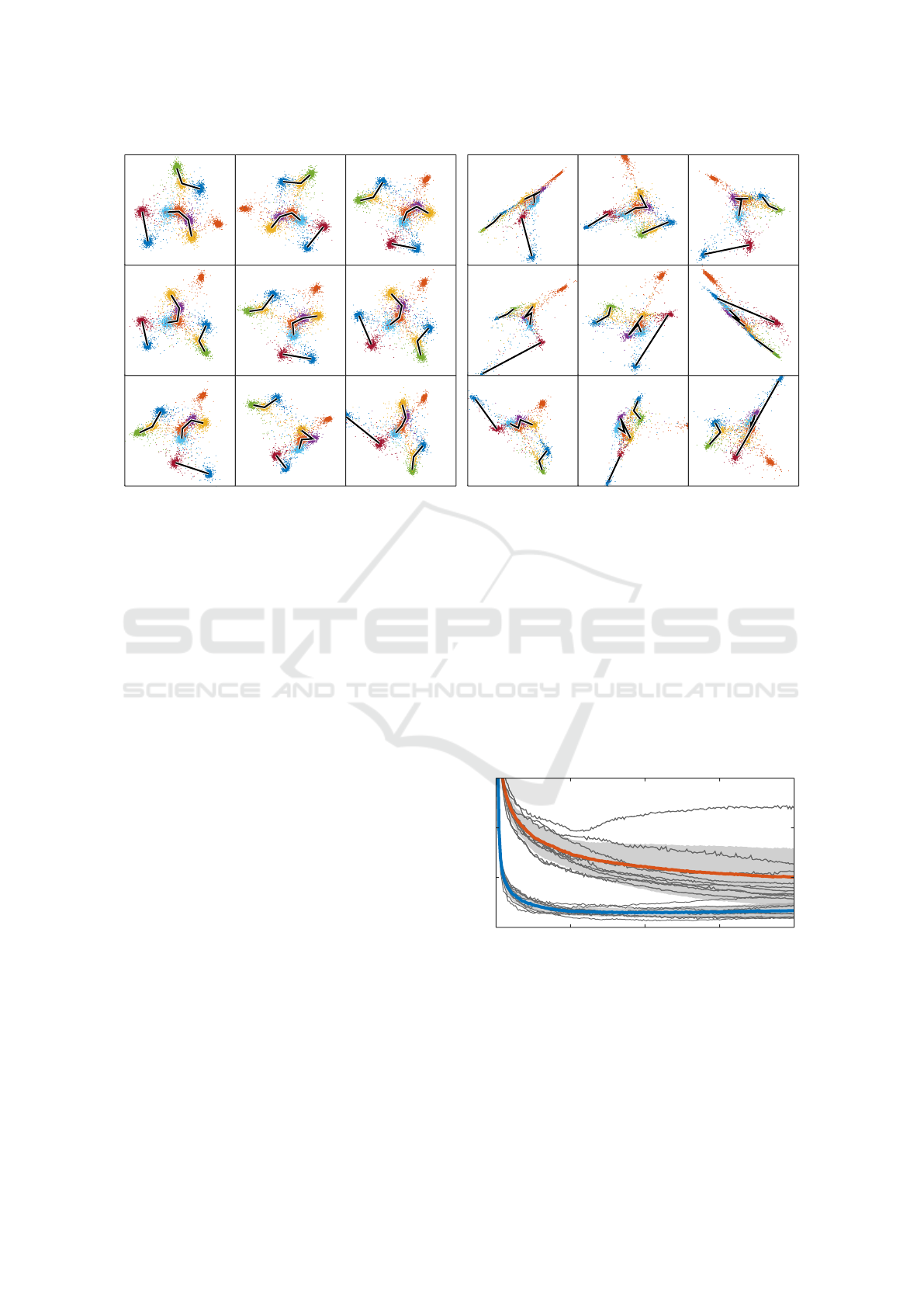
3.2.2 2D Visualization
In the following we demonstrate ReNDA’s improved
robustness compared to GerDA by two means: We
use 2D scatter plots for data visualization and the
class consistency measure DSC suggested by (Sips
et al., 2009) to assess the quality and the robustness
of the underlying 2D mappings.
The scatter plots in Figure 4(a) show the results of
the 9 ReNDA runs. Each column corresponds to 1 of
the 3 partitions of the 60k training samples and each
row corresponds to 1 of the 3 random number streams
as described in the previous section. The 2D features
depicted are based on the 10k validation samples of
the respective run. Figure 4(b) shows the associated
GerDA scatter plots and it is organized in the very
same way. This includes that two scatter plots with
same position in 4(a) and 4(b) are based on the same
combination of a training set partition and a random
number stream.
The value given in the bottom left corner of each
scatter plot is the associated DSC score. DSC = 100
means that all data points have a smaller Euclidean
Table 1: A comparison of the DSC scores of several DNN
approaches to 2D feature extraction from the MNIST data
set. The validation results (average ± standard deviation)
for ReNDA and GerDA are based on the 9 DSCs shown
in Figure 4(a) and 4(b), respectively. For both ReNDA
and GerDA, the test results were obtained by applying the
f
enc
associated with the best validation DSC score on the
10k test samples. In order not only to compare ReNDA
and GerDA, we ran all 9 experiments with a deep belief
net DNN (DBN-DNN) approach suggested by (Tanaka and
Okutomi, 2014) (cf. Section 3.2.5). Additionally, the lower
table shows the comparison presented by (Stuhlsatz et al.,
2012). Here, no validation results were stated.
Our new results
Learned model Validation Test
ReNDA 94.94 ± 0.39 95.03
GerDA 91.47 ± 3.03 93.49
DBN-DNN
∗
96.62 ± 0.22 96.67
DBN-DNN + LDA
∗
93.78 ± 4.66 97.00
∗
) cf. Section 3.2.5
Formerly published results
Learned model Validation Test
t-SNE n/a 88.99
NNCA n/a 95.03
GerDA n/a 96.83
distance their own class centroid than to any other. It
is a good measure of visual class separability that can
be directly applied to any low-dimensional features
even if the underlying original sets of samples are not
available. Table 1 presents a comparison of the DSC
scores of ReNDA, GerDA and three other approaches
to dimensionality reduction for data visualization. Of
course, the fact that (Stuhlsatz et al., 2012) achieved
a higher DSC score is a less positive result. However,
considering the rather high standard deviation within
our 9 GerDA runs, this DSC score appears to be a
bit misleading, i.e. significantly lower DSC scores are
very likely to occur. It is easy to see that ReNDA is
much more reliable as regards the DSC score.
Less evident is the fact that ReNDA again yields
reliably reproducible feature mappings. To illustrate
that this is nevertheless the case, we suggest a fictive
walk through each of ReNDA’s scatter plots:
We start at 1 in any scatter plot and walk through
the corridor formed by the two clusters 2-3-8-5 and
7-9-4. Note that [except in the column 2, row 3 plot]
both these clusters are arc-shaped or, more precisely,
curved towards the path that we are walking on. We
stop midway between 4 and 5 and then turn in the
direction of the 2-3-8-5 cluster. From here, [except in
the column 1, row 2 plot] we first see 6 and then 0.
Here, standing at 0 we would be able to see the other
side of the 2-3-8-5 arc.
IVAPP 2017 - International Conference on Information Visualization Theory and Applications
122
95.24
0
0
0
0
0
0
0
0
0
0
0
0
0
00
0
0
0
0
0
0
0
0
0
0
0
0
0
1
1
1
1
1
1
1
1
1
1
1
1
1
11
1
1
1
1
1
1
1
1
1
1
1
1
1
2
2
2
2
2
2
2
2
2
2
2
2
2
22
2
2
2
2
2
2
2
2
2
2
2
2
2
3
3
3
3
3
3
3
3
3
3
3
3
3
33
3
3
3
3
3
3
3
3
3
3
3
3
3
4
4
4
4
4
4
4
4
4
4
4
4
4
44
4
4
4
4
4
4
4
4
4
4
4
4
4
5
5
5
5
5
5
5
5
5
5
5
5
5
55
5
5
5
5
5
5
5
5
5
5
5
5
5
6
6
6
6
6
6
6
6
6
6
6
6
6
66
6
6
6
6
6
6
6
6
6
6
6
6
6
7
7
7
7
7
7
7
7
7
7
7
7
7
77
7
7
7
7
7
7
7
7
7
7
7
7
7
8
8
8
8
8
8
8
8
8
8
8
8
8
88
8
8
8
8
8
8
8
8
8
8
8
8
8
9
9
9
9
9
9
9
9
9
9
9
9
9
99
9
9
9
9
9
9
9
9
9
9
9
9
9
94.99
0
0
0
0
0
0
0
0
0
0
0
0
0
00
0
0
0
0
0
0
0
0
0
0
0
0
0
1
1
1
1
1
1
1
1
1
1
1
1
1
11
1
1
1
1
1
1
1
1
1
1
1
1
1
2
2
2
2
2
2
2
2
2
2
2
2
2
22
2
2
2
2
2
2
2
2
2
2
2
2
2
3
3
3
3
3
3
3
3
3
3
3
3
3
33
3
3
3
3
3
3
3
3
3
3
3
3
3
4
4
4
4
4
4
4
4
4
4
4
4
4
44
4
4
4
4
4
4
4
4
4
4
4
4
4
5
5
5
5
5
5
5
5
5
5
5
5
5
55
5
5
5
5
5
5
5
5
5
5
5
5
5
6
6
6
6
6
6
6
6
6
6
6
6
6
66
6
6
6
6
6
6
6
6
6
6
6
6
6
7
7
7
7
7
7
7
7
7
7
7
7
7
77
7
7
7
7
7
7
7
7
7
7
7
7
7
8
8
8
8
8
8
8
8
8
8
8
8
8
88
8
8
8
8
8
8
8
8
8
8
8
8
8
9
9
9
9
9
9
9
9
9
9
9
9
9
99
9
9
9
9
9
9
9
9
9
9
9
9
9
94.52
0
0
0
0
0
0
0
0
0
0
0
0
0
00
0
0
0
0
0
0
0
0
0
0
0
0
0
1
1
1
1
1
1
1
1
1
1
1
1
1
11
1
1
1
1
1
1
1
1
1
1
1
1
1
2
2
2
2
2
2
2
2
2
2
2
2
2
22
2
2
2
2
2
2
2
2
2
2
2
2
2
3
3
3
3
3
3
3
3
3
3
3
3
3
33
3
3
3
3
3
3
3
3
3
3
3
3
3
4
4
4
4
4
4
4
4
4
4
4
4
4
44
4
4
4
4
4
4
4
4
4
4
4
4
4
5
5
5
5
5
5
5
5
5
5
5
5
5
55
5
5
5
5
5
5
5
5
5
5
5
5
5
6
6
6
6
6
6
6
6
6
6
6
6
6
66
6
6
6
6
6
6
6
6
6
6
6
6
6
7
7
7
7
7
7
7
7
7
7
7
7
7
77
7
7
7
7
7
7
7
7
7
7
7
7
7
8
8
8
8
8
8
8
8
8
8
8
8
8
88
8
8
8
8
8
8
8
8
8
8
8
8
8
9
9
9
9
9
9
9
9
9
9
9
9
9
99
9
9
9
9
9
9
9
9
9
9
9
9
9
95.21
0
0
0
0
0
0
0
0
0
0
0
0
0
00
0
0
0
0
0
0
0
0
0
0
0
0
0
1
1
1
1
1
1
1
1
1
1
1
1
1
11
1
1
1
1
1
1
1
1
1
1
1
1
1
2
2
2
2
2
2
2
2
2
2
2
2
2
22
2
2
2
2
2
2
2
2
2
2
2
2
2
3
3
3
3
3
3
3
3
3
3
3
3
3
33
3
3
3
3
3
3
3
3
3
3
3
3
3
4
4
4
4
4
4
4
4
4
4
4
4
4
44
4
4
4
4
4
4
4
4
4
4
4
4
4
5
5
5
5
5
5
5
5
5
5
5
5
5
55
5
5
5
5
5
5
5
5
5
5
5
5
5
6
6
6
6
6
6
6
6
6
6
6
6
6
66
6
6
6
6
6
6
6
6
6
6
6
6
6
7
7
7
7
7
7
7
7
7
7
7
7
7
77
7
7
7
7
7
7
7
7
7
7
7
7
7
8
8
8
8
8
8
8
8
8
8
8
8
8
88
8
8
8
8
8
8
8
8
8
8
8
8
8
9
9
9
9
9
9
9
9
9
9
9
9
9
99
9
9
9
9
9
9
9
9
9
9
9
9
9
95.44
0
0
0
0
0
0
0
0
0
0
0
0
0
00
0
0
0
0
0
0
0
0
0
0
0
0
0
1
1
1
1
1
1
1
1
1
1
1
1
1
11
1
1
1
1
1
1
1
1
1
1
1
1
1
2
2
2
2
2
2
2
2
2
2
2
2
2
22
2
2
2
2
2
2
2
2
2
2
2
2
2
3
3
3
3
3
3
3
3
3
3
3
3
3
33
3
3
3
3
3
3
3
3
3
3
3
3
3
4
4
4
4
4
4
4
4
4
4
4
4
4
44
4
4
4
4
4
4
4
4
4
4
4
4
4
5
5
5
5
5
5
5
5
5
5
5
5
5
55
5
5
5
5
5
5
5
5
5
5
5
5
5
6
6
6
6
6
6
6
6
6
6
6
6
6
66
6
6
6
6
6
6
6
6
6
6
6
6
6
7
7
7
7
7
7
7
7
7
7
7
7
7
77
7
7
7
7
7
7
7
7
7
7
7
7
7
8
8
8
8
8
8
8
8
8
8
8
8
8
88
8
8
8
8
8
8
8
8
8
8
8
8
8
9
9
9
9
9
9
9
9
9
9
9
9
9
99
9
9
9
9
9
9
9
9
9
9
9
9
9
94.97
0
0
0
0
0
0
0
0
0
0
0
0
0
00
0
0
0
0
0
0
0
0
0
0
0
0
0
1
1
1
1
1
1
1
1
1
1
1
1
1
11
1
1
1
1
1
1
1
1
1
1
1
1
1
2
2
2
2
2
2
2
2
2
2
2
2
2
22
2
2
2
2
2
2
2
2
2
2
2
2
2
3
3
3
3
3
3
3
3
3
3
3
3
3
33
3
3
3
3
3
3
3
3
3
3
3
3
3
4
4
4
4
4
4
4
4
4
4
4
4
4
44
4
4
4
4
4
4
4
4
4
4
4
4
4
5
5
5
5
5
5
5
5
5
5
5
5
5
55
5
5
5
5
5
5
5
5
5
5
5
5
5
6
6
6
6
6
6
6
6
6
6
6
6
6
66
6
6
6
6
6
6
6
6
6
6
6
6
6
7
7
7
7
7
7
7
7
7
7
7
7
7
77
7
7
7
7
7
7
7
7
7
7
7
7
7
8
8
8
8
8
8
8
8
8
8
8
8
8
88
8
8
8
8
8
8
8
8
8
8
8
8
8
9
9
9
9
9
9
9
9
9
9
9
9
9
99
9
9
9
9
9
9
9
9
9
9
9
9
9
95.01
0
0
0
0
0
0
0
0
0
0
0
0
0
00
0
0
0
0
0
0
0
0
0
0
0
0
0
1
1
1
1
1
1
1
1
1
1
1
1
1
11
1
1
1
1
1
1
1
1
1
1
1
1
1
2
2
2
2
2
2
2
2
2
2
2
2
2
22
2
2
2
2
2
2
2
2
2
2
2
2
2
3
3
3
3
3
3
3
3
3
3
3
3
3
33
3
3
3
3
3
3
3
3
3
3
3
3
3
4
4
4
4
4
4
4
4
4
4
4
4
4
44
4
4
4
4
4
4
4
4
4
4
4
4
4
5
5
5
5
5
5
5
5
5
5
5
5
5
55
5
5
5
5
5
5
5
5
5
5
5
5
5
6
6
6
6
6
6
6
6
6
6
6
6
6
66
6
6
6
6
6
6
6
6
6
6
6
6
6
7
7
7
7
7
7
7
7
7
7
7
7
7
77
7
7
7
7
7
7
7
7
7
7
7
7
7
8
8
8
8
8
8
8
8
8
8
8
8
8
88
8
8
8
8
8
8
8
8
8
8
8
8
8
9
9
9
9
9
9
9
9
9
9
9
9
9
99
9
9
9
9
9
9
9
9
9
9
9
9
9
94.89
0
0
0
0
0
0
0
0
0
0
0
0
0
00
0
0
0
0
0
0
0
0
0
0
0
0
0
1
1
1
1
1
1
1
1
1
1
1
1
1
11
1
1
1
1
1
1
1
1
1
1
1
1
1
2
2
2
2
2
2
2
2
2
2
2
2
2
22
2
2
2
2
2
2
2
2
2
2
2
2
2
3
3
3
3
3
3
3
3
3
3
3
3
3
33
3
3
3
3
3
3
3
3
3
3
3
3
3
4
4
4
4
4
4
4
4
4
4
4
4
4
44
4
4
4
4
4
4
4
4
4
4
4
4
4
5
5
5
5
5
5
5
5
5
5
5
5
5
55
5
5
5
5
5
5
5
5
5
5
5
5
5
6
6
6
6
6
6
6
6
6
6
6
6
6
66
6
6
6
6
6
6
6
6
6
6
6
6
6
7
7
7
7
7
7
7
7
7
7
7
7
7
77
7
7
7
7
7
7
7
7
7
7
7
7
7
8
8
8
8
8
8
8
8
8
8
8
8
8
88
8
8
8
8
8
8
8
8
8
8
8
8
8
9
9
9
9
9
9
9
9
9
9
9
9
9
99
9
9
9
9
9
9
9
9
9
9
9
9
9
94.16
0
0
0
0
0
0
0
0
0
0
0
0
0
00
0
0
0
0
0
0
0
0
0
0
0
0
0
1
1
1
1
1
1
1
1
1
1
1
1
1
11
1
1
1
1
1
1
1
1
1
1
1
1
1
2
2
2
2
2
2
2
2
2
2
2
2
2
22
2
2
2
2
2
2
2
2
2
2
2
2
2
3
3
3
3
3
3
3
3
3
3
3
3
3
33
3
3
3
3
3
3
3
3
3
3
3
3
3
4
4
4
4
4
4
4
4
4
4
4
4
4
44
4
4
4
4
4
4
4
4
4
4
4
4
4
5
5
5
5
5
5
5
5
5
5
5
5
5
55
5
5
5
5
5
5
5
5
5
5
5
5
5
6
6
6
6
6
6
6
6
6
6
6
6
6
66
6
6
6
6
6
6
6
6
6
6
6
6
6
7
7
7
7
7
7
7
7
7
7
7
7
7
77
7
7
7
7
7
7
7
7
7
7
7
7
7
8
8
8
8
8
8
8
8
8
8
8
8
8
88
8
8
8
8
8
8
8
8
8
8
8
8
8
9
9
9
9
9
9
9
9
9
9
9
9
9
99
9
9
9
9
9
9
9
9
9
9
9
9
9
(a) 2D mappings learned by ReNDA
89.57
0
0
0
0
0
0
0
0
0
0
0
0
0
00
0
0
0
0
0
0
0
0
0
0
0
0
0
1
1
1
1
1
1
1
1
1
1
1
1
1
11
1
1
1
1
1
1
1
1
1
1
1
1
1
2
2
2
2
2
2
2
2
2
2
2
2
2
22
2
2
2
2
2
2
2
2
2
2
2
2
2
3
3
3
3
3
3
3
3
3
3
3
3
3
33
3
3
3
3
3
3
3
3
3
3
3
3
3
4
4
4
4
4
4
4
4
4
4
4
4
4
44
4
4
4
4
4
4
4
4
4
4
4
4
4
5
5
5
5
5
5
5
5
5
5
5
5
5
55
5
5
5
5
5
5
5
5
5
5
5
5
5
6
6
6
6
6
6
6
6
6
6
6
6
6
66
6
6
6
6
6
6
6
6
6
6
6
6
6
7
7
7
7
7
7
7
7
7
7
7
7
7
77
7
7
7
7
7
7
7
7
7
7
7
7
7
8
8
8
8
8
8
8
8
8
8
8
8
8
88
8
8
8
8
8
8
8
8
8
8
8
8
8
9
9
9
9
9
9
9
9
9
9
9
9
9
99
9
9
9
9
9
9
9
9
9
9
9
9
9
92.45
0
0
0
0
0
0
0
0
0
0
0
0
0
00
0
0
0
0
0
0
0
0
0
0
0
0
0
1
1
1
1
1
1
1
1
1
1
1
1
1
11
1
1
1
1
1
1
1
1
1
1
1
1
1
2
2
2
2
2
2
2
2
2
2
2
2
2
22
2
2
2
2
2
2
2
2
2
2
2
2
2
3
3
3
3
3
3
3
3
3
3
3
3
3
33
3
3
3
3
3
3
3
3
3
3
3
3
3
4
4
4
4
4
4
4
4
4
4
4
4
4
44
4
4
4
4
4
4
4
4
4
4
4
4
4
5
5
5
5
5
5
5
5
5
5
5
5
5
55
5
5
5
5
5
5
5
5
5
5
5
5
5
6
6
6
6
6
6
6
6
6
6
6
6
6
66
6
6
6
6
6
6
6
6
6
6
6
6
6
7
7
7
7
7
7
7
7
7
7
7
7
7
77
7
7
7
7
7
7
7
7
7
7
7
7
7
8
8
8
8
8
8
8
8
8
8
8
8
8
88
8
8
8
8
8
8
8
8
8
8
8
8
8
9
9
9
9
9
9
9
9
9
9
9
9
9
99
9
9
9
9
9
9
9
9
9
9
9
9
9
92.59
0
0
0
0
0
0
0
0
0
0
0
0
0
00
0
0
0
0
0
0
0
0
0
0
0
0
0
1
1
1
1
1
1
1
1
1
1
1
1
1
11
1
1
1
1
1
1
1
1
1
1
1
1
1
2
2
2
2
2
2
2
2
2
2
2
2
2
22
2
2
2
2
2
2
2
2
2
2
2
2
2
3
3
3
3
3
3
3
3
3
3
3
3
3
33
3
3
3
3
3
3
3
3
3
3
3
3
3
4
4
4
4
4
4
4
4
4
4
4
4
4
44
4
4
4
4
4
4
4
4
4
4
4
4
4
5
5
5
5
5
5
5
5
5
5
5
5
5
55
5
5
5
5
5
5
5
5
5
5
5
5
5
6
6
6
6
6
6
6
6
6
6
6
6
6
66
6
6
6
6
6
6
6
6
6
6
6
6
6
7
7
7
7
7
7
7
7
7
7
7
7
7
77
7
7
7
7
7
7
7
7
7
7
7
7
7
8
8
8
8
8
8
8
8
8
8
8
8
8
88
8
8
8
8
8
8
8
8
8
8
8
8
8
9
9
9
9
9
9
9
9
9
9
9
9
9
99
9
9
9
9
9
9
9
9
9
9
9
9
9
93.2
0
0
0
0
0
0
0
0
0
0
0
0
0
00
0
0
0
0
0
0
0
0
0
0
0
0
0
1
1
1
1
1
1
1
1
1
1
1
1
1
11
1
1
1
1
1
1
1
1
1
1
1
1
1
2
2
2
2
2
2
2
2
2
2
2
2
2
22
2
2
2
2
2
2
2
2
2
2
2
2
2
3
3
3
3
3
3
3
3
3
3
3
3
3
33
3
3
3
3
3
3
3
3
3
3
3
3
3
4
4
4
4
4
4
4
4
4
4
4
4
4
44
4
4
4
4
4
4
4
4
4
4
4
4
4
5
5
5
5
5
5
5
5
5
5
5
5
5
55
5
5
5
5
5
5
5
5
5
5
5
5
5
6
6
6
6
6
6
6
6
6
6
6
6
6
66
6
6
6
6
6
6
6
6
6
6
6
6
6
7
7
7
7
7
7
7
7
7
7
7
7
7
77
7
7
7
7
7
7
7
7
7
7
7
7
7
8
8
8
8
8
8
8
8
8
8
8
8
8
88
8
8
8
8
8
8
8
8
8
8
8
8
8
9
9
9
9
9
9
9
9
9
9
9
9
9
99
9
9
9
9
9
9
9
9
9
9
9
9
9
92.8
0
0
0
0
0
0
0
0
0
0
0
0
0
00
0
0
0
0
0
0
0
0
0
0
0
0
0
1
1
1
1
1
1
1
1
1
1
1
1
1
11
1
1
1
1
1
1
1
1
1
1
1
1
1
2
2
2
2
2
2
2
2
2
2
2
2
2
22
2
2
2
2
2
2
2
2
2
2
2
2
2
3
3
3
3
3
3
3
3
3
3
3
3
3
33
3
3
3
3
3
3
3
3
3
3
3
3
3
4
4
4
4
4
4
4
4
4
4
4
4
4
44
4
4
4
4
4
4
4
4
4
4
4
4
4
5
5
5
5
5
5
5
5
5
5
5
5
5
55
5
5
5
5
5
5
5
5
5
5
5
5
5
6
6
6
6
6
6
6
6
6
6
6
6
6
66
6
6
6
6
6
6
6
6
6
6
6
6
6
7
7
7
7
7
7
7
7
7
7
7
7
7
77
7
7
7
7
7
7
7
7
7
7
7
7
7
8
8
8
8
8
8
8
8
8
8
8
8
8
88
8
8
8
8
8
8
8
8
8
8
8
8
8
9
9
9
9
9
9
9
9
9
9
9
9
9
99
9
9
9
9
9
9
9
9
9
9
9
9
9
84.06
0
0
0
0
0
0
0
0
0
0
0
0
0
00
0
0
0
0
0
0
0
0
0
0
0
0
0
1
1
1
1
1
1
1
1
1
1
1
1
1
11
1
1
1
1
1
1
1
1
1
1
1
1
1
2
2
2
2
2
2
2
2
2
2
2
2
2
22
2
2
2
2
2
2
2
2
2
2
2
2
2
3
3
3
3
3
3
3
3
3
3
3
3
3
33
3
3
3
3
3
3
3
3
3
3
3
3
3
4
4
4
4
4
4
4
4
4
4
4
4
4
44
4
4
4
4
4
4
4
4
4
4
4
4
4
5
5
5
5
5
5
5
5
5
5
5
5
5
55
5
5
5
5
5
5
5
5
5
5
5
5
5
6
6
6
6
6
6
6
6
6
6
6
6
6
66
6
6
6
6
6
6
6
6
6
6
6
6
6
7
7
7
7
7
7
7
7
7
7
7
7
7
77
7
7
7
7
7
7
7
7
7
7
7
7
7
8
8
8
8
8
8
8
8
8
8
8
8
8
88
8
8
8
8
8
8
8
8
8
8
8
8
8
9
9
9
9
9
9
9
9
9
9
9
9
9
99
9
9
9
9
9
9
9
9
9
9
9
9
9
93.72
0
0
0
0
0
0
0
0
0
0
0
0
0
00
0
0
0
0
0
0
0
0
0
0
0
0
0
1
1
1
1
1
1
1
1
1
1
1
1
1
11
1
1
1
1
1
1
1
1
1
1
1
1
1
2
2
2
2
2
2
2
2
2
2
2
2
2
22
2
2
2
2
2
2
2
2
2
2
2
2
2
3
3
3
3
3
3
3
3
3
3
3
3
3
33
3
3
3
3
3
3
3
3
3
3
3
3
3
4
4
4
4
4
4
4
4
4
4
4
4
4
44
4
4
4
4
4
4
4
4
4
4
4
4
4
5
5
5
5
5
5
5
5
5
5
5
5
5
55
5
5
5
5
5
5
5
5
5
5
5
5
5
6
6
6
6
6
6
6
6
6
6
6
6
6
66
6
6
6
6
6
6
6
6
6
6
6
6
6
7
7
7
7
7
7
7
7
7
7
7
7
7
77
7
7
7
7
7
7
7
7
7
7
7
7
7
8
8
8
8
8
8
8
8
8
8
8
8
8
88
8
8
8
8
8
8
8
8
8
8
8
8
8
9
9
9
9
9
9
9
9
9
9
9
9
9
99
9
9
9
9
9
9
9
9
9
9
9
9
9
93.11
0
0
0
0
0
0
0
0
0
0
0
0
0
00
0
0
0
0
0
0
0
0
0
0
0
0
0
1
1
1
1
1
1
1
1
1
1
1
1
1
11
1
1
1
1
1
1
1
1
1
1
1
1
1
2
2
2
2
2
2
2
2
2
2
2
2
2
22
2
2
2
2
2
2
2
2
2
2
2
2
2
3
3
3
3
3
3
3
3
3
3
3
3
3
33
3
3
3
3
3
3
3
3
3
3
3
3
3
4
4
4
4
4
4
4
4
4
4
4
4
4
44
4
4
4
4
4
4
4
4
4
4
4
4
4
5
5
5
5
5
5
5
5
5
5
5
5
5
55
5
5
5
5
5
5
5
5
5
5
5
5
5
6
6
6
6
6
6
6
6
6
6
6
6
6
66
6
6
6
6
6
6
6
6
6
6
6
6
6
7
7
7
7
7
7
7
7
7
7
7
7
7
77
7
7
7
7
7
7
7
7
7
7
7
7
7
8
8
8
8
8
8
8
8
8
8
8
8
8
88
8
8
8
8
8
8
8
8
8
8
8
8
8
9
9
9
9
9
9
9
9
9
9
9
9
9
99
9
9
9
9
9
9
9
9
9
9
9
9
9
91.73
0
0
0
0
0
0
0
0
0
0
0
0
0
00
0
0
0
0
0
0
0
0
0
0
0
0
0
1
1
1
1
1
1
1
1
1
1
1
1
1
11
1
1
1
1
1
1
1
1
1
1
1
1
1
2
2
2
2
2
2
2
2
2
2
2
2
2
22
2
2
2
2
2
2
2
2
2
2
2
2
2
3
3
3
3
3
3
3
3
3
3
3
3
3
33
3
3
3
3
3
3
3
3
3
3
3
3
3
4
4
4
4
4
4
4
4
4
4
4
4
4
44
4
4
4
4
4
4
4
4
4
4
4
4
4
5
5
5
5
5
5
5
5
5
5
5
5
5
55
5
5
5
5
5
5
5
5
5
5
5
5
5
6
6
6
6
6
6
6
6
6
6
6
6
6
66
6
6
6
6
6
6
6
6
6
6
6
6
6
7
7
7
7
7
7
7
7
7
7
7
7
7
77
7
7
7
7
7
7
7
7
7
7
7
7
7
8
8
8
8
8
8
8
8
8
8
8
8
8
88
8
8
8
8
8
8
8
8
8
8
8
8
8
9
9
9
9
9
9
9
9
9
9
9
9
9
99
9
9
9
9
9
9
9
9
9
9
9
9
9
(b) 2D mappings learned by GerDA
Figure 4: A comparison of the 2D mappings learned by ReNDA (a) and GerDA (b). In both (a) and (b) the class centroids
are marked with the associated digits. Furthermore, clusters of digit classes are indicated by solid black lines. Each column
corresponds to 1 of the 3 partitions of the training samples and each row corresponds to 1 of the 3 random number streams.
The DSC score of each experiment is placed in the lower left corner.
This walk example shows that relative positions
of the classes to each other are very similar from plot
to plot. So in conclusion, the simulated fluctuations
merely result in rotations and mirrorings of otherwise
very similar scatter plots. In the the corresponding
GerDA scatter plots (cf. Figure 4(b)), we were unable
to visually detect such a high degree of similarity. It
again follows that ReNDA is better regularized than
GerDA.
3.2.3 Robust Learning Behavior
It is natural to assume that the above final results are
due to a more robust, more efficient and more targeted
learning behavior. To test this, we compare the two
learning curves depicted in Figure 5. The curves show
the validation classification error (error for short) as
a function of learning epochs, the iterative steps of
DNN learning. Clearly, like the DSC score, the error
is a measure of class separability. The reason why we
use it here is to show ReNDA also performs well on
classification tasks.
In detail, we see the average ReNDA error (lower
emphasized, blue curve) and the average GerDA error
(upper emphasized, red curve). Both are surrounded
by a light gray ribbon indicating the corresponding
standard deviation per epoch. The thinner dark gray
curves represent the errors of the 9 ReNDA and the 9
GerDA runs, respectively.
Here, the assumed more robust learning behavior
of ReNDA is evident because throughout all learning
epochs its standard deviation is significantly smaller
than that of GerDA. Also its average learning curve
is almost constant after epoch 50 whereas GerDA’s
average learning curve is still falling at epoch 200,
which surely can be interpreted as a more efficient and
more targeted learning behavior.
0 50 100 150 200
4
8
12
16
Figure 5: A comparison of the learning curves associated
with ReNDA and GerDA. Each learning curve shows the
validation classification error (error for short) as a function
of the learning epoch. The lower blue and the upper red
curve represent the average errors. The light gray ribbon
surrounding each of the two indicates the corresponding
standard deviations per epoch. The thinner dark gray curves
show the actual errors per epoch of the 9 ReNDA runs and
the 9 GerDA runs.
Regularized Nonlinear Discriminant Analysis - An Approach to Robust Dimensionality Reduction for Data Visualization
123
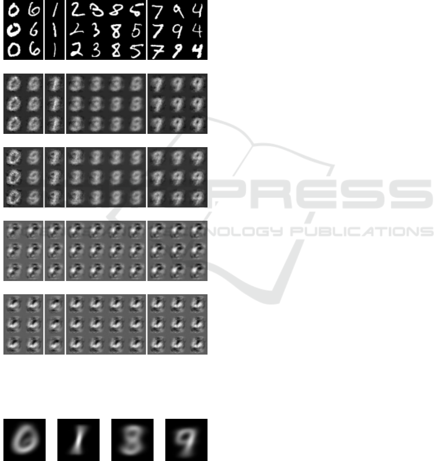
3.2.4 DAE Reconstruction
In the previous two subsections, we only compared
ReNDA and GerDA concerning their robustness. To
that end, we looked at 2D scatter plots, DSC scores
and learning curves, i.e. views and measures directly
associated with the extracted features Z. We will now
have a look at the data reconstructions
b
X that can be
(a) Original MNIST test samples.
(b) ReNDA, best DSC score
(c) ReNDA, worst DSC score
(d) GerDA, best DSC score
(e) GerDA, worst DSC score
Figure 6: Reconstructions of the MNIST test images, where
(a) shows the original samples. The digits are grouped as in
Figure 4: 0-6, 1, 2-3-8-5 and 7-9-4. The details on (b) to (e)
are given in Section 3.2.4.
(a) 0-6 (b) 1 (c) 2-3-8-5 (d) 7-9-4
Figure 7: Average images of all test samples associated with
the four clusters 0-6 (a), 1 (b), 2-3-8-5 (c) and 7-9-4 (d) as
depicted in Figure 4.
obtained from this features.
For the reconstructions in Figure 6(b) ReNDA’s
encoder mapping f
enc
with the best validation DSC
score and its associated decoder mapping f
dec
were
applied on the MNIST test images. For Figure 6(c)
we did the same but with ReNDA’s worst f
enc
and its
associated f
dec
. Observe that digits lying in the 7-9-4
cluster have a reconstruction that looks like a blurry
9. In the case of the 2-3-8-5 cluster, it is very similar
but with a blurry 3. Clearly, this shows that f
dec
is
able to decode features in a meaningful way, which
can be further supported by looking at the means of
these clusters (cf. Figure 7). As a matter of fact, the
mean images of the 7-9-4 and the 2-3-8-5 cluster are
a blurry 9 and a blurry 3, respectively. Another aspect
is that these blurry 9s and 3s do not vary much from
Figure 6(b) to Figure 6(c). It follows that the decoder
mappings are also very robust, which is certainly due
to the parameter sharing introduced via (12) and (13)
(cf. Section 2.2).
The “reconstructions” shown in Figure 6(d) and
Figure 6(e) are based on the GerDA runs with the
best and the worst validation DSC score. In order to
be able to decode the features, a decoding DNN has
been constructed from the learned encoding GerDA
DNN via (12) and (13), ReNDA’s parameter sharing
relations. Further, we have set b
b
b
2L
= 0
0
0. The result
clearly shows that DNN learning of a GerDA DNN
generally does not yield suitable network parameters
for decoding. At the same time, we have proven that
the quality of ReNDA’s reconstructions are in fact due
to DNN learning of the decoder DNN with respect to
the combined criterion J
ReNDA
(cf. (2)).
A closer investigation reveals that the images in
Figure 6(d) are different to those in Figure 6(e) which
again indicates that GerDA is not as well-regularized
as ReNDA. A very fascinating result is that all digit
reconstructions of each of the two GerDA runs appear
to be identical, i.e. a learned GerDA DNN assigns the
same reconstruction to all digits when constructing a
decoder via (12) and (13). The investigation of this
phenomenon is a part of our future work.
3.2.5 Comparison with Another DNN
So far, we have only compared ReNDA to its direct
predecessor GerDA. In order to be able to provide
further comparisons, we ran our 9 experiments with
the deep belief net DNN (DBN-DNN) approach that
has been suggested by (Tanaka and Okutomi, 2014).
Though originally designed to infer a binary target
vector scheme y 7→ t
t
t ∈ {0,1}
C
given by
t
i
(y) =
(
1 i = y
0 i 6= y
y ∈ {1,...,C}, (25)
IVAPP 2017 - International Conference on Information Visualization Theory and Applications
124
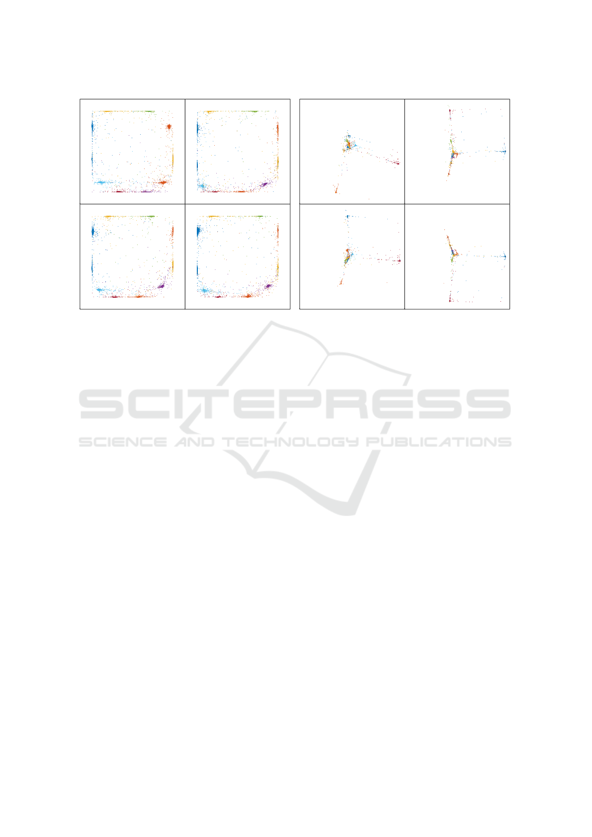
96.72
0
0
0
0
0
0
0
0
0
0
0
0
0
00
0
0
0
0
0
0
0
0
0
0
0
0
0
1
1
1
1
1
1
1
1
1
1
1
1
1
11
1
1
1
1
1
1
1
1
1
1
1
1
1
2
2
2
2
2
2
2
2
2
2
2
2
2
22
2
2
2
2
2
2
2
2
2
2
2
2
2
3
3
3
3
3
3
3
3
3
3
3
3
3
33
3
3
3
3
3
3
3
3
3
3
3
3
3
4
4
4
4
4
4
4
4
4
4
4
4
4
44
4
4
4
4
4
4
4
4
4
4
4
4
4
5
5
5
5
5
5
5
5
5
5
5
5
5
55
5
5
5
5
5
5
5
5
5
5
5
5
5
6
6
6
6
6
6
6
6
6
6
6
6
6
66
6
6
6
6
6
6
6
6
6
6
6
6
6
7
7
7
7
7
7
7
7
7
7
7
7
7
77
7
7
7
7
7
7
7
7
7
7
7
7
7
8
8
8
8
8
8
8
8
8
8
8
8
8
88
8
8
8
8
8
8
8
8
8
8
8
8
8
9
9
9
9
9
9
9
9
9
9
9
9
9
99
9
9
9
9
9
9
9
9
9
9
9
9
9
96.64
0
0
0
0
0
0
0
0
0
0
0
0
0
00
0
0
0
0
0
0
0
0
0
0
0
0
0
1
1
1
1
1
1
1
1
1
1
1
1
1
11
1
1
1
1
1
1
1
1
1
1
1
1
1
2
2
2
2
2
2
2
2
2
2
2
2
2
22
2
2
2
2
2
2
2
2
2
2
2
2
2
3
3
3
3
3
3
3
3
3
3
3
3
3
33
3
3
3
3
3
3
3
3
3
3
3
3
3
4
4
4
4
4
4
4
4
4
4
4
4
4
44
4
4
4
4
4
4
4
4
4
4
4
4
4
5
5
5
5
5
5
5
5
5
5
5
5
5
55
5
5
5
5
5
5
5
5
5
5
5
5
5
6
6
6
6
6
6
6
6
6
6
6
6
6
66
6
6
6
6
6
6
6
6
6
6
6
6
6
7
7
7
7
7
7
7
7
7
7
7
7
7
77
7
7
7
7
7
7
7
7
7
7
7
7
7
8
8
8
8
8
8
8
8
8
8
8
8
8
88
8
8
8
8
8
8
8
8
8
8
8
8
8
9
9
9
9
9
9
9
9
9
9
9
9
9
99
9
9
9
9
9
9
9
9
9
9
9
9
9
96.77
0
0
0
0
0
0
0
0
0
0
0
0
0
00
0
0
0
0
0
0
0
0
0
0
0
0
0
1
1
1
1
1
1
1
1
1
1
1
1
1
11
1
1
1
1
1
1
1
1
1
1
1
1
1
2
2
2
2
2
2
2
2
2
2
2
2
2
22
2
2
2
2
2
2
2
2
2
2
2
2
2
3
3
3
3
3
3
3
3
3
3
3
3
3
33
3
3
3
3
3
3
3
3
3
3
3
3
3
4
4
4
4
4
4
4
4
4
4
4
4
4
44
4
4
4
4
4
4
4
4
4
4
4
4
4
5
5
5
5
5
5
5
5
5
5
5
5
5
55
5
5
5
5
5
5
5
5
5
5
5
5
5
6
6
6
6
6
6
6
6
6
6
6
6
6
66
6
6
6
6
6
6
6
6
6
6
6
6
6
7
7
7
7
7
7
7
7
7
7
7
7
7
77
7
7
7
7
7
7
7
7
7
7
7
7
7
8
8
8
8
8
8
8
8
8
8
8
8
8
88
8
8
8
8
8
8
8
8
8
8
8
8
8
9
9
9
9
9
9
9
9
9
9
9
9
9
99
9
9
9
9
9
9
9
9
9
9
9
9
9
96.57
0
0
0
0
0
0
0
0
0
0
0
0
0
00
0
0
0
0
0
0
0
0
0
0
0
0
0
1
1
1
1
1
1
1
1
1
1
1
1
1
11
1
1
1
1
1
1
1
1
1
1
1
1
1
2
2
2
2
2
2
2
2
2
2
2
2
2
22
2
2
2
2
2
2
2
2
2
2
2
2
2
3
3
3
3
3
3
3
3
3
3
3
3
3
33
3
3
3
3
3
3
3
3
3
3
3
3
3
4
4
4
4
4
4
4
4
4
4
4
4
4
44
4
4
4
4
4
4
4
4
4
4
4
4
4
5
5
5
5
5
5
5
5
5
5
5
5
5
55
5
5
5
5
5
5
5
5
5
5
5
5
5
6
6
6
6
6
6
6
6
6
6
6
6
6
66
6
6
6
6
6
6
6
6
6
6
6
6
6
7
7
7
7
7
7
7
7
7
7
7
7
7
77
7
7
7
7
7
7
7
7
7
7
7
7
7
8
8
8
8
8
8
8
8
8
8
8
8
8
88
8
8
8
8
8
8
8
8
8
8
8
8
8
9
9
9
9
9
9
9
9
9
9
9
9
9
99
9
9
9
9
9
9
9
9
9
9
9
9
9
(a) 2D mappings learned by DBN-DNN
96.62
0
0
0
0
0
0
0
0
0
0
0
0
0
00
0
0
0
0
0
0
0
0
0
0
0
0
0
1
1
1
1
1
1
1
1
1
1
1
1
1
11
1
1
1
1
1
1
1
1
1
1
1
1
1
2
2
2
2
2
2
2
2
2
2
2
2
2
22
2
2
2
2
2
2
2
2
2
2
2
2
2
3
3
3
3
3
3
3
3
3
3
3
3
3
33
3
3
3
3
3
3
3
3
3
3
3
3
3
4
4
4
4
4
4
4
4
4
4
4
4
4
44
4
4
4
4
4
4
4
4
4
4
4
4
4
5
5
5
5
5
5
5
5
5
5
5
5
5
55
5
5
5
5
5
5
5
5
5
5
5
5
5
6
6
6
6
6
6
6
6
6
6
6
6
6
66
6
6
6
6
6
6
6
6
6
6
6
6
6
7
7
7
7
7
7
7
7
7
7
7
7
7
77
7
7
7
7
7
7
7
7
7
7
7
7
7
8
8
8
8
8
8
8
8
8
8
8
8
8
88
8
8
8
8
8
8
8
8
8
8
8
8
8
9
9
9
9
9
9
9
9
9
9
9
9
9
99
9
9
9
9
9
9
9
9
9
9
9
9
9
97.12
0
0
0
0
0
0
0
0
0
0
0
0
0
00
0
0
0
0
0
0
0
0
0
0
0
0
0
1
1
1
1
1
1
1
1
1
1
1
1
1
11
1
1
1
1
1
1
1
1
1
1
1
1
1
2
2
2
2
2
2
2
2
2
2
2
2
2
22
2
2
2
2
2
2
2
2
2
2
2
2
2
3
3
3
3
3
3
3
3
3
3
3
3
3
33
3
3
3
3
3
3
3
3
3
3
3
3
3
4
4
4
4
4
4
4
4
4
4
4
4
4
44
4
4
4
4
4
4
4
4
4
4
4
4
4
5
5
5
5
5
5
5
5
5
5
5
5
5
55
5
5
5
5
5
5
5
5
5
5
5
5
5
6
6
6
6
6
6
6
6
6
6
6
6
6
66
6
6
6
6
6
6
6
6
6
6
6
6
6
7
7
7
7
7
7
7
7
7
7
7
7
7
77
7
7
7
7
7
7
7
7
7
7
7
7
7
8
8
8
8
8
8
8
8
8
8
8
8
8
88
8
8
8
8
8
8
8
8
8
8
8
8
8
9
9
9
9
9
9
9
9
9
9
9
9
9
99
9
9
9
9
9
9
9
9
9
9
9
9
9
97.10
0
0
0
0
0
0
0
0
0
0
0
0
0
00
0
0
0
0
0
0
0
0
0
0
0
0
0
1
1
1
1
1
1
1
1
1
1
1
1
1
11
1
1
1
1
1
1
1
1
1
1
1
1
1
2
2
2
2
2
2
2
2
2
2
2
2
2
22
2
2
2
2
2
2
2
2
2
2
2
2
2
3
3
3
3
3
3
3
3
3
3
3
3
3
33
3
3
3
3
3
3
3
3
3
3
3
3
3
4
4
4
4
4
4
4
4
4
4
4
4
4
44
4
4
4
4
4
4
4
4
4
4
4
4
4
5
5
5
5
5
5
5
5
5
5
5
5
5
55
5
5
5
5
5
5
5
5
5
5
5
5
5
6
6
6
6
6
6
6
6
6
6
6
6
6
66
6
6
6
6
6
6
6
6
6
6
6
6
6
7
7
7
7
7
7
7
7
7
7
7
7
7
77
7
7
7
7
7
7
7
7
7
7
7
7
7
8
8
8
8
8
8
8
8
8
8
8
8
8
88
8
8
8
8
8
8
8
8
8
8
8
8
8
9
9
9
9
9
9
9
9
9
9
9
9
9
99
9
9
9
9
9
9
9
9
9
9
9
9
9
87.86
0
0
0
0
0
0
0
0
0
0
0
0
0
00
0
0
0
0
0
0
0
0
0
0
0
0
0
1
1
1
1
1
1
1
1
1
1
1
1
1
11
1
1
1
1
1
1
1
1
1
1
1
1
1
2
2
2
2
2
2
2
2
2
2
2
2
2
22
2
2
2
2
2
2
2
2
2
2
2
2
2
3
3
3
3
3
3
3
3
3
3
3
3
3
33
3
3
3
3
3
3
3
3
3
3
3
3
3
4
4
4
4
4
4
4
4
4
4
4
4
4
44
4
4
4
4
4
4
4
4
4
4
4
4
4
5
5
5
5
5
5
5
5
5
5
5
5
5
55
5
5
5
5
5
5
5
5
5
5
5
5
5
6
6
6
6
6
6
6
6
6
6
6
6
6
66
6
6
6
6
6
6
6
6
6
6
6
6
6
7
7
7
7
7
7
7
7
7
7
7
7
7
77
7
7
7
7
7
7
7
7
7
7
7
7
7
8
8
8
8
8
8
8
8
8
8
8
8
8
88
8
8
8
8
8
8
8
8
8
8
8
8
8
9
9
9
9
9
9
9
9
9
9
9
9
9
99
9
9
9
9
9
9
9
9
9
9
9
9
9
(b) 2D mappings learned by DBN-DNN + LDA
Figure 8: A comparison of the 2D mappings learned by the DBN-DNN (a) and the DBN-DNN + LDA (b). As in Figure 4
the class centroids are marked with the associated digits. Each column corresponds to first 2 of 3 partitions of the training
samples and each row corresponds to first 2 of 3 random number streams. DSC scores are placed in the lower right corner.
we expected it to yield informative, visualizable 2D
features. We designed two DBN-DNN experiments,
each of which involves the same 9 runs that we used
for our ReNDA and GerDA experiments, i.e. we again
considered each combination of the 3 partitions of the
training samples with the 3 random number streams.
Figures 8(a) and 8(b) show the obtained 2D features
associated with the 10k validation samples. Because
the within class scatter is very small compared to
the between class scatter, we decided to show only
the four plots corresponding to the first 2 partitions
and the first 2 random number streams, respectively.
However, the validation results given in Table 1 are
based on all 9 runs. The details on the experimental
setup can be found in Appendix D.
In our first experiment, we changed the original
topology 784-1200-1200-10 (Tanaka and Okutomi,
2014) into 784-1200-1200-2-10, i.e. the intermediate
dimension 2 was added in order to obtain visualizable
features. As can be seen, the 2D mappings are highly
reproducible and the corresponding DSC scores are
slightly higher than those of ReNDA. A surprising
fact is that the visually separable 2D features tend
to lie close to the rim of product set (0|1) × (0|1).
Surely, these particular feature bounds are due to our
choice of activation functions: We used sigm : R →
(0|1) for all DBN-DNN layers. But the concentration
of the features at the rim of the feature space remains
an open question.
In our second experiment, we used the original
topology 784-1200-1200-10 for DNN learning and
applied a classical LDA : R
10
→ R
2
dimensionality
reduction, afterwards. We refer to this approach as
DBN-DNN + LDA (cf. Table 1). Although the DSC
scores of the obtained 2D mappings are even higher
than those of the above DBN-DNN experiment, the
corresponding scatter plots are quiet different to each
other. We can therefore conclude that this approach
is not as well-regularized as the DBN-DNN and the
ReNDA approach. The details on the experimental
setup of the DBN-DNN + LDA experiment are given
in Appendix D.
4 CONCLUSION
In this paper, we presented and investigated a novel
approach to robust dimensionality reduction for data
visualization that is a combination of two DNNs: One
is a nonlinear generalization of Fisher’s LDA called
GerDA (Stuhlsatz et al., 2012). The other DNN is a
deep autoencoder (DAE) (Hinton and Salakhutdinov,
2006). We refer to the combined DNN as ReNDA
(Regularized Nonlinear Discriminant Analysis). In
the context of data visualization, a well-regularized
DNN guarantees to learn a reliably reproducible 1D,
2D or 3D feature representation.
In order to test ReNDAs reliability, we designed
extensive experiments with simulated fluctuations in
the data. We presented various data visualizations to
Regularized Nonlinear Discriminant Analysis - An Approach to Robust Dimensionality Reduction for Data Visualization
125

show that the learned dimensionality reductions are
very useful for information visualization and visual
data mining. Here, ReNDA has shown to be more
robust against the simulated data fluctuations than
GerDA. As far as we know, this paper is the first to
present such extensive experiments on the robustness
of DNNs. Therefore, we were forced to run all the
experiments on our own. Our experiments with the
DBN-DNN provide a first glance at the capability of
another approach to dimensionality reduction for data
visualization (cf. Section 3.2.5). Of course, there are
other DNN approaches that are capable of learning
informative, visualizable features but here, one must
have in mind that extensive experiments are essential
to the process of finding suitable DNNs.
In this context, an important task is to figure out
what we can learn from other suitable DNNs, e.g. the
DBN-DNN (Tanaka and Okutomi, 2014). One of our
future task will be to include the recently proposed
drop out regularization (Srivastava et al., 2014). In
addition to the investigation and integration of other
promising approaches, there are of course some open
questions within the ReNDA approach itself: The
most important is if there is a better value for λ than
0.5 and if there is a way to automatically determine
an optimal λ-value. The next question points out a
chance that comes with ReNDA: Can we exploit the
unsupervised learning that the DAE part of ReNDA
performs, so that semi-supervised learning tasks can
be handled?
In summary, ReNDA has been shown to provide
a good way of learning dimensionality reductions for
data visualization. Moreover, questions like the two
above clearly show that the ReNDA approach can be
further advanced and adapted to suit a wide range of
real-world applications. Providing the possibility to
use ReNDA for semi-supervised learning will be an
essential advancement in this context.
ACKNOWLEDGEMENTS
We would like to thank the OVGU Magdeburg, the
Faculty of Media (HS D
¨
usseldorf) and the Faculty of
Mechanical and Process Engineering (HS D
¨
usseldorf)
for providing us with the computational power for our
extensive experiments.
REFERENCES
Duda, R. O., Hart, P. E., and Stork, D. G. (2000). Pattern
Classification. John Wiley & Sons, Inc.
Erhan, D., Bengio, Y., Courville, A., Manzagol, P.-A.,
and Vincent, P. (2010). Why does unsupervised pre-
training help deep learning? Journal of Machine
Learning Research, 11:625–660.
Fisher, R. A. (1936). The use of multiple measurements in
taxonomic problems. Annals of Eugenics, 7:179–188.
Hinton, G. E. and Salakhutdinov, R. R. (2006). Reducing
the dimensionality of data with neural networks. SCI-
ENCE, 313:504–507.
LeCun, Y., Bottou, L., Bengio, Y., and Haffner, P. (1998).
Gradient-based learning applied to document recogni-
tion. Proc. of the IEEE, pages 1–46.
Sips, M., Neubert, B., Lewis, J. P., and Hanrahan, P. (2009).
Selecting good views of high-dimensional data us-
ing class consistency. Computer Graphics Forum,
28(3):831–838.
Srivastava, N., Hinton, G., Krizhevsky, A., Sutskever, I.,
and Salakhutdinov, R. (2014). Dropout: A simple way
to prevent neural networks from overfitting. Journal
of Machine Learning Research, 15:1929–1958.
Stuhlsatz, A., Lippel, J., and Zielke, T. (2012). Feature ex-
traction with deep neural networks by a generalized
discriminant analysis. IEEE Transactions on Neural
Networks, 666:1–666.
Stuhlsatz, A., Meyer, C., Eyben, F., ZieIke, T., Meier,
G., and Schuller, B. (2011). Deep neural networks
for acoustic emotion recognition: Raising the bench-
marks. In Proc. IEEE Intern. Conf. on Acoustics,
Speech and Signal Processing (ICASSP).
Tanaka, M. (2016). Deep neural network. MATLAB Central
File Exchange (# 42853). Retrieved Dec 2016.
Tanaka, M. and Okutomi, M. (2014). A novel inference
of a restricted boltzmann machine. In 22nd Inter-
national Conference on Pattern Recognition, ICPR
2014, Stockholm, Sweden, August 24-28, 2014, pages
1526–1531.
Zhai, Y., Ong, Y. S., and Tsang, I. W. (2014). The emerg-
ing ”big dimensionality”. IEEE Computational Intel-
ligence Magazine, 9(3):14–26.
APPENDIX
A. On the Normalized GerDA Criterion
In Section 2.4.1, we stated that the GerDA criterion
(21) is normalized, i.e. that J
GerDA
∈ (0|1). As this
is not straightforward to see, we give a proof in this
appendix section.
Let λ
k
for k ∈ {1,...,d
Z
} denote the eigenvalues
of (S
δ
T
)
−1
S
δ
B
. Then trace
(S
δ
T
)
−1
S
δ
B
=
∑
n
k=1
λ
k
and
we need to show that 0 < λ
k
< 1 for all k.
Therefore, let µ
k
for k ∈ {1,...,d
Z
} denote the
eigenvalues of S
−1
W
S
δ
B
and let x
x
x
k
∈ R
d
Z
denote an
eigenvector to the eigenvalue µ
k
. Then
S
−1
W
S
δ
B
x
x
x
k
= µ
k
x
x
x
k
⇔ x
x
x
tr
k
S
δ
B
x
x
x
k
= µ
k
· x
x
x
tr
k
S
W
x
x
x
k
.
(26)
IVAPP 2017 - International Conference on Information Visualization Theory and Applications
126

Since both S
δ
B
and S
W
(cf. (19) and (20)) are positive
definite, we have that µ
k
> 0 for all k. We use (18) to
rewrite the characteristic eigenvalue equation associ-
ated with (26) as follows:
S
−1
W
S
δ
B
− µ
k
I
d
Z
x
x
x
k
= 0
0
0
⇔
S
−1
W
(S
δ
T
− S
W
) − µ
k
I
d
Z
x
x
x
k
= 0
0
0
⇔
S
−1
W
S
δ
T
− (µ
k
+ 1)
| {z }
=:κ
k
I
d
Z
x
x
x
k
= 0
0
0 (27)
Clearly, κ
k
for k ∈ {1,...,d
Z
} denote the eigenvalues
of S
−1
W
S
δ
T
and it is κ
k
> 1 for all k. The eigenvalues
of (S
−1
W
S
δ
T
)
−1
are simply 0 < κ
−1
k
< 1 for all k. We
finally use that (S
−1
W
S
δ
T
)
−1
= I
d
Z
−(S
δ
T
)
−1
S
δ
B
which is
equivalent to (18). With these last two statements we
further convert (27) to
⇔
(S
−1
W
S
δ
T
)
−1
− κ
−1
k
I
d
Z
x
x
x
k
= 0
0
0
⇔
(S
δ
T
)
−1
S
δ
B
−
1 − κ
−1
k
| {z }
=λ
k
I
d
Z
x
x
x
k
= 0
0
0. (28)
Here, it is easy to see that 0 < λ
k
< 1 for all k, which
is what we intended to show.
B. Partial Derivatives of J
GerDA
Let ` ∈ {1,.. .,L}. The partial derivatives of J
GerDA
(cf. (21)) are given by
∂J
GerDA
∂W
`
= ∆
∆
∆
`
(X
`−1
)
tr
(29)
∂J
GerDA
∂b
b
b
`
= ∆
∆
∆
`
· 1
1
1
N
(30)
with 1
1
1
N
:= (1,1,. .., 1)
tr
∈ R
N
and
∆
∆
∆
`
:= f
0
`
(A
`
)
(
∂J
GerDA
/∂Z ` = L
(W
`+1
)
tr
∆
∆
∆
`+1
1 ≤ ` < L .
(31)
It is
∂J
GerDA
∂Z
= −
1
d
Z
·
∂Q
δ
z
∂Z
. (32)
A computable expression for ∂Q
δ
z
/∂Z along with its
derivation is given in (Stuhlsatz et al., 2012).
C. Partial Derivatives of J
DAE
In the case of J
DAE
(cf. (24)), the partial derivatives
with respect to the weight matrices are given by
∂J
DAE
∂W
`
= Λ
Λ
Λ
`
(X
`−1
)
tr
+
Λ
Λ
Λ
2L−`+1
(X
2L−`
)
tr
tr
(33)
for ` ∈ {1,...L}. The partial derivatives with respect
to the bias vectors are given by
∂J
DAE
∂b
`
=
(
Λ
Λ
Λ
2L
· 1
1
1
N
` = 2L
(Λ
Λ
Λ
`
+ Λ
Λ
Λ
2L−`
) · 1
1
1
N
1 ≤ ` < L .
(34)
with 1
1
1
N
:= (1,...,1)
tr
∈ R
N
. For ` ∈ {1,...2L} the
matrices Λ
Λ
Λ
`
are defined by
Λ
Λ
Λ
`
:= f
0
`
(A
`
)
(
∂J
DAE
/∂
b
X ` = 2L
(W
`+1
)
tr
Λ
Λ
Λ
`+1
1 ≤ ` < 2L .
(35)
with
∂J
DAE
∂
b
X
=
2
b
X − X
d
X
· N · (1 + MSE/d
X
)
, (36)
which is straightforward to prove.
D. Data Presentation for DNN Learning
The following table contains the details for our exper-
iments with the galaxy data sets and the MNIST data
set.
Table 2: Summary of our experiments details: In the case
of ReNDA and GerDA, batchsizes and number of epochs
were chosen as in (Stuhlsatz et al., 2012). In the case of the
DBN-DNN approach, we simply used the default settings
from the code provided by (Tanaka, 2016).
ReNDA and GerDA
Setup / Property Galaxy MNIST
Data dimensionality 2 784
Feature dimensionality 1 2
Number of classes 3 10
Number of data samples
used for DNN learning 1440 50000
used for validation 5118 10000
total, distinct 65580 60000
Pretraining
Batchsize 144 2000
Number of Epochs 10 50
Fine-tuning
Batchsize 288 5000
Number of Epochs 1000 200
DBN-DNN and DBN-DNN + LDA
∗
Pretraining
Batchsize 100
Number of Epochs 1000
Fine-tuning
Batchsize 100
Number of Epochs 1000
(
∗
) only the differences to the ReNDA / GerDA experiments
Regularized Nonlinear Discriminant Analysis - An Approach to Robust Dimensionality Reduction for Data Visualization
127
