Visualizing Temporal Graphs using Visual Rhythms
A Case Study in Soccer Match Analysis
Daniele C. Uchoa Maia Rodrigues
1
, Felipe A. Moura
2
,
Sergio Augusto Cunha
3
and Ricardo da S. Torres
1
1
Institute of Computing, University of Campinas, Campinas, Brazil
2
Laboratory of Applied Biomechanics, State University of Londrina, Londrina, Brazil
3
College of Physical Education, University of Campinas, Campinas, Brazil
Keywords:
Visual Rhythm, Temporal Graph, Complex Network, Soccer Analysis.
Abstract:
In several applications, a huge amount of graph data have been generated, demanding the creation of appropri-
ate tools for graph visualization. One class of graph data which is attracting a lot of attention recently are the
temporal graphs, which encode how objects and their relationships evolve over time. This paper introduces
the Graph Visual Rhythm, a novel image-based representation to visualize changing patterns typically found
in temporal graphs. The use of visual rhythms is motivated by its capacity of providing a lot of contextual
information about graph dynamics in a compact way. We validate the use of graph visual rhythms through the
creation of a visual analytics tool to support the decision-making process based on complex-network-oriented
soccer match analysis.
1 INTRODUCTION
Huge volumes of graph data have been generated in
several applications, demanding the development of
appropriate tools for storing, processing, and anal-
ysis. Examples of applications include social net-
work (Zhao and Tung, 2012; Brandes et al., 2012),
sport analysis (Duch et al., 2010; Cotta et al., 2013;
Pe
˜
na and Touchette, 2012; Passos et al., 2011), and
urban planing (Nahman and Peri, 2017). One partic-
ular class of graphs that is attracting a lot of attention
recently are the temporal graphs, which basically rep-
resent the insertion and deletion of vertices and edges
over time (Leskovec et al., 2005).
In this paper, we are interested in visually repre-
senting temporal graphs, with the objective of sup-
porting the identification and analysis of temporal
pattern changes. In this context, several approaches
have been proposed to the visualization of tempo-
ral graphs (Brandes and Corman, 2003; Hurter et al.,
2014; Brandes et al., 2012; Beck et al., 2016). Most
of the approaches rely on the use of node-link dia-
grams, where different visual marks (typically circle
glyphs) are used for representing vertices and lines to
visually represent relations among vertices. Differ-
ent additional visual properties associated with visual
marks (e.g., position, size, length, angle, slope, color,
gray scale, texture, shape, animation, blink, motion)
are employed to highlight properties associated with
both vertices and edges (Beck et al., 2016). A typical
challenge faced by those initiatives refers to the visu-
alization of huge volumes of data. In these scenarios,
complex interaction controls have been proposed to
handle occlusion and to support browsing activities
over graph data.
In this paper, we address this problem from a
different perspective. We propose a graph-to-image
transformation, so that large volumes of sequence
graphs can be visually represented in a compact way,
enabling fast and easy visual identification of pattern
changes. Our solution relies on the use of the visual
rhythm representation (Ngo et al., 1999). This ap-
proach has been typically used for efficient video data
processing and analysis (Bezerra and Lima, 2006;
da Silva Pinto et al., 2015), as it allows the repre-
sentation of the whole video content by means of an
image, whose columns are defined by the extraction
of features from pixels of frames. In this paper, we
extend this idea by encoding properties of graph se-
quences, leading to a representation we name graph
visual rhythm. For each instant of time, graph proper-
ties are represented as a column of an image, allowing
the compact representation of important graph fea-
tures associated with changes of vertices and edges
96
C. Uchoa Maia Rodrigues D., A. Moura F., Cunha S. and da S. Torres R.
Visualizing Temporal Graphs using Visual Rhythms - A Case Study in Soccer Match Analysis.
DOI: 10.5220/0006153000960107
In Proceedings of the 12th International Joint Conference on Computer Vision, Imaging and Computer Graphics Theory and Applications (VISIGRAPP 2017), pages 96-107
ISBN: 978-989-758-228-8
Copyright
c
 2017 by SCITEPRESS – Science and Technology Publications, Lda. All rights reserved

over time. Our solution is somehow similar to pre-
vious initiatives focusing on encoding graph dynam-
ics using matrix representations (Burch et al., 2011;
Vehlow et al., 2013; Bach et al., 2014). Different
from those initiatives, however, our approach does not
rely on radial layouts, nor on complex representations
such as small multiples and stacked matrices. To the
best of our knowledge, this is the first attempt to en-
code complex temporal graph changes in a easy-to-
interpret single image representation.
The proposed method is validated in the context
of soccer match analysis. Recently, sport science re-
searchers have been dedicated to the representation of
soccer match events by means of graphs (Duch et al.,
2010; Cotta et al., 2013; Pe
˜
na and Touchette, 2012;
Passos et al., 2011). Usually, players are represented
as vertices and their relations (e.g., passes, proxim-
ity) are encoded as edges. In some of those applica-
tions, graph properties, defined in terms of complex
network topological measures are used in the match
analysis. In this paper, we describe the use of graph
visual rhythms defined in terms of complex network
measures for understanding complex temporal pat-
terns associated with the match dynamics.
In summary, the contributions of this paper are
twofold: (i) the introduction of a novel compact vi-
sual representation for temporal graphs, named graph
visual rhythm; and (ii) the presentation of different
scenarios of its use in the context of the analysis of
real soccer matches using complex network measures.
2 BACKGROUND
2.1 Visual Rhythms
Visual Rhythm is a sampling method widely used
to video processing and analysis (Ngo et al., 1999;
Guimar
˜
aes et al., 2003; Chun et al., 2002). Its ob-
jective is to transform tridimensional information into
bidimensional images by sampling one dimensional
information from video frames. Let V be a digital
video (in domain 2D + t) composed of T frames f
t
,
i.e., V = ( f
t
), t ∈ [1, T ], where T is the number of
frames. Let H and W be, respectively, the height and
width from each frame f
t
.
The visual rhythm computation consists in using a
function to map each f
t
into a column of an image in
domain 1D+t. The final image generated is known as
visual rhythm image (VR). More formally, the com-
putation of the VR image is defined as follows (Ngo
et al., 1999; Guimar
˜
aes et al., 2003):
V R(t, z) = f
t
(r
x
× z + a, r
y
× z + b), (1)
!!
!!
Height!(H)!
Height!(H)!
Width!(T)!
Width!(W)!
Time!(T)!
Figure 1: Example of visual rhythm computed by extracting
the pixel values defined by the central vertical line. In this
example, r
x
= 1, r
y
= 0, a = 0, and b =
W
2
. This leads
to a visual rhythm V R = f
t
(z,
W
2
), where z ∈ [1, H
V R
] and
t ∈ [1, T ], H
V R
= H is the height of the visual rhythm image,
and T is its width.
where z ∈ [1, H
V R
] and t ∈ [1, T ], H
V R
and T are the
height (i.e., H
V R
= H) and the width of the visual
rhythm image; r
x
and r
y
are ratios of pixel sampling; a
and b are shifts on each frame. Figure 1 illustrates the
computation of visual rhythm based on the pixel val-
ues defined by the vertical line passing in the center
of the frame.
A more general definition of visual rhythms as-
sumes that it is possible to use a function F to
represent each frame of a video as point in an n-
dimensional space. Let f
t
be a frame defined in
terms of D, a set of pixels. Function F is defined as
F : D → R
n
. For example, a widely used implemen-
tation of function F relies on the computation of the
histogram associated with each frame f
t
(Guimar
˜
aes
et al., 2003). In this case, the visual rhythm image is
a 2D representation encoding all frame histograms as
vertical lines, i.e.,
V R(t, z) = H ( f
t
), (2)
where H ( f
t
) is a function that computes the his-
togram of frame f
t
, t ∈ [1, T ] and z ∈ [1, L], T is
the number of frames and L the number of histogram
bins.
2.2 Complex Network Measurements
Soccer is one of the most difficult sports to analyze
quantitatively due to the complexity of the play and
to the nearly uninterrupted flow of the ball during
the match. Indeed, unlike other sports, in which in-
dividual game-related statistics may properly repre-
sent player performance, in soccer it is not trivial to
define quantitative measures of an individual contri-
bution (Duch et al., 2010). Moreover, simple statis-
tics such as number of assists or number of shots may
not provide a reliable measure of a player’s true im-
pact on team performance and, consequently, the out-
comes of a match (Duch et al., 2010; Moura et al.,
Visualizing Temporal Graphs using Visual Rhythms - A Case Study in Soccer Match Analysis
97

2014). Instead, the real contribution of a given player
sometimes is hidden in the plays of the team, such
as participating from a passing sequence to a shot on
goal (Duch et al., 2010). This type of information is
important to detail the role of a team member on team
performance. Thus, this study uses complex network
measurements for extracting features from graphs to
represent individual behavior and thus to represent
team performance using a visual analytical tool. Two
measurements were considered in this work: Diver-
sity Entropy and Betweenness Centrality.
2.2.1 Diversity Entropy
The dynamic aspects associated with passes among
players in a match (such as the ‘ball flow’ among the
players of a team) are important cues for game tacti-
cal analysis (Duch et al., 2010). In this paper, we use
the diversity entropy (Travenc¸olo and Costa, 2008;
Travenc¸olo et al., 2009) as a variable to characterize
the dynamic nature of the match, characterizing the
possibility of passes among players.
Diversity Entropy considers the transition proba-
bility (P
h
( j, i)) that a node i reaches a node j after h
steps in a self avoiding random walk. Let Ω be the set
of all nodes but i. The normalized diversity entropy
of a node i is defined as (Travenc¸olo et al., 2009):
E
h
(Ω, i) = −
1
log(N − 1)
N
∑
j=1

P
h
( j, i)log(P
h
( j, i)), if P
h
( j, i) 6= 0,
0, if P
h
( j, i) = 0.
(3)
2.2.2 Betweenness Centrality
In this paper, the centrality of players in a match is re-
lated to his role in the passing flow along the time. We
used betweenness centrality to characterize the role
of players in terms of the graph shortest paths with
which the players are involved.
Betweenness centrality (Costa et al., 2007) of a
node u is quantified as the sum over all distinct pairs
of vertex i, j of the number of shortest paths from i to
j that pass through u (θ(i, u, j)) divided by the total
number of shortest paths between i and j (θ(i, j)):
B
u
=
∑
i j
θ(i, u, j)
θ(i, j )
(4)
3 GRAPH VISUAL RHYTHMS
We define a temporal graph G as a sequence G =
hG
1
, G
2
, . . . , G
T
i, where G
t
= (V
t
, E
t
) is a weighted
graph at timestamp t ∈ [1, T ] composed of a set of
vertices, V
t
, and a set of edges, E
t
. We refer to the
graph defined at a particular timestamp t (say G
t
) as
1
3
5
8
1
3
5
8
V4
V1 V1 V1
V2 V2
V2
V3 V3
V3
V4
V4
V5
time
V1 V2 V3 V4
0.0 0.5 1.0 1.5 2.0 2.5 3.0
V1 V2 V3 V4
0.0 0.5 1.0 1.5 2.0 2.5 3.0
V1 V2 V3 V4 V5
0 1 2 3 4
. . .
2
2
3
1
0
2
3
3
2
0
2
3
4
2
1
. . .
. . .
V5
V1
V4
V3
V2
V5
V4
V3
V2
V1
Vertex Degree Vertex Degree Vertex Degree
A
A
A
B B B
C
V1
V2
V3
V4
1
2
3
0
0
1
2
3
0
V1
V2
V3
V4
1
2
3
0
4
V1
V2
V3
V4 V5
Width (T)
Height (H)
t
n
t
n
t
2
t
1
t
1
t
2
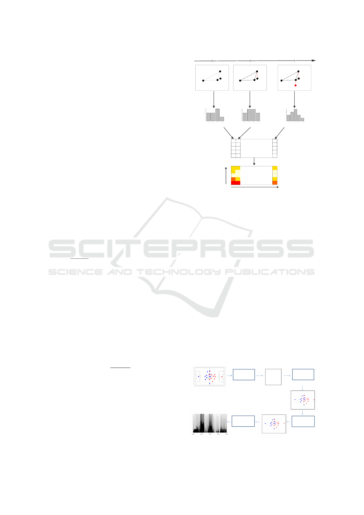
Figure 2: Flowchart illustrating how a graph visual rhythm
is extracted.
an instant graph. By building one graph for each in-
stant of time considering the vertices’ interaction, it is
possible to capture the temporal nature of the graph
dynamics. Our goal is to represent the interaction
among vertices at each instant using a visual rhythm
representation GV R. We follow a similar formulation
employed in Eq. 2 to define GV R:
GV R(t, z) = F (G
t
), (5)
where F
G
t
: G → R
n
is a function that represents a
graph G
t
∈ G as a point in an n-dimensional space,
t ∈ [1, T ] and z ∈ [1, n].
Figure 2 illustrates the computation of a graph vi-
sual rhythm for a temporal graph. Changes in the
graph sequence are highlighted in red. For example,
at timestamp t
2
, an edge linking vertices v
2
and v
4
is
created. At timestamp t
n
, vertex v
5
is created along
with an edge from v
5
to v
3
. In this example, function
F
G
t
computes the degree of vertices for each instant
of time (arrows labeled with A). The degree informa-
tion is later used to create the graph visual rhythm
Visual Graph Rhythm
Image Computation
(d)
Complex Network
Measure Computation
(c)
0.55
0.35
0.35
0.35
0.40
0.80
Players’ Location
Extraction
(a)
GraphExtraction
(b)
99.598 33.6378
73.646 46.1074
75.5410 19.6833
79.6112 33.3785
67.6252 27.5689
56.8979 9.6359
67.4589 35.2626
Figure 3: Analysis framework.
IVAPP 2017 - International Conference on Information Visualization Theory and Applications
98

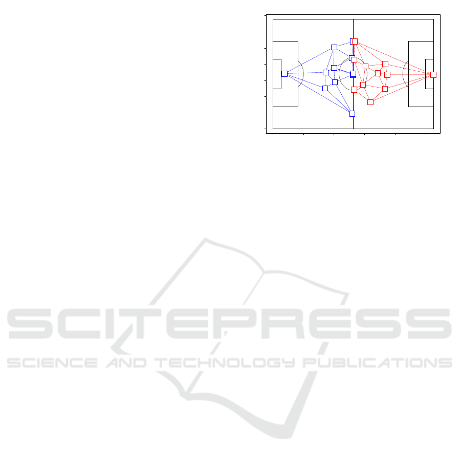
image (arrows B). Again different visual properties
(e.g., color, opacity) may be used to highlight graph
changes. In the case of the example, a heatmap-based
color layout is employed (arrow C).
4 CASE STUDY: SOCCER MATCH
ANALYSIS
This study is based on the use of graph visual rhythms
for identifying events on temporal graphs associated
with soccer matches.
4.1 Soccer Match Analysis Framework
The graph-based soccer match analysis framework
employed in this study comprises four steps, as illus-
trated in Figure 3:
(a) Extraction of players’ location in field over time:
This step is accomplished using the DVideo soft-
ware (Figueroa et al., 2006a; Figueroa et al.,
2006b) applied to official soccer matches. This
process starts with soccer match videos and re-
sults in files containing players xy location on
the pitch and annotation related to match events,
such as passes accomplished, fouls, shots on goal,
among others. The extraction frame rate is 30
frames per second, so for a typical 45-minute half
time of a match, we have 81,000 frames. We used
a dataset related to two official soccer matches (re-
ferred to as Match 1 and Match 2 along the paper)
of the Brazilian Professional First League Cham-
pionship.
(b) Graph Extraction: This step builds graphs from
soccer match frames. In our experiments, two
different kinds of graphs were built: Delaunay
Triangulation Instant Graphs and Flow Networks,
which are detailed in Section 4.2.
(c) Complex Network Measure Computation: This
step comprises the approach described in Sec-
tion 2.2. Basically, complex network measures
are computed from graphs obtained in Step b. In
this experiment, two measures were considered:
Diversity Entropy and Betweeness Centrality. In
this context, these measures are extracted by F
G
t
,
the function that encodes one graph into a column
of a graph visual rhythm.
(d) Visual Graph Rhythm Image Computation: This
step is concerned with the creation of graph vi-
sual rhythm images. From those images, it is
possible to analyze patterns that represent match
events such as attacking and defensive strategies
from each team.
0 20 40 60 80 100
0 10 20 30 40 50 60 70
x
y
Graph Plot − Frame: 10
1
2
3
4
5
6
7
8
9
10
11
15
16
17
18
19
20
21
22
23
24
25
1
2
3
4
5
6
7
8
9
10
11
15
16
17
18
19
20
21
22
23
24
25
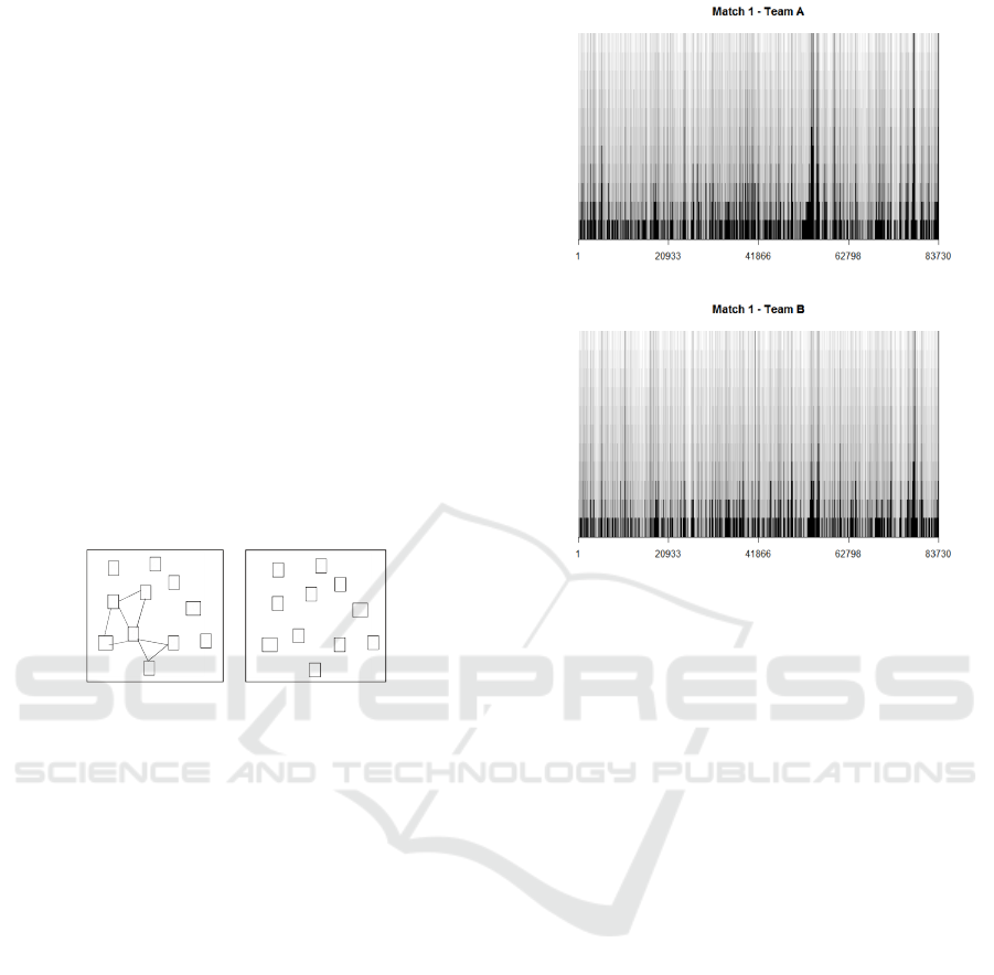
Figure 4: Examples of Delaunay Triangulation instant
graphs of two teams (represented in blue and red).
4.2 Soccer Temporal Graphs
Our analyses are based on the characterization of in-
teraction among players along the match. Let G
0
be
a sequence G
0
= hG
1
, G
2
, . . . , G
T
i. A vertex v ∈ V
t
is associated with a player, whereas an edge e
jk
∈ E
t
connecting two vertices v
j
∈ E
t
and v
k
∈ E
t
is defined
based on the location (or any other relation) of play-
ers (v
j
and v
k
) of the same team at timestamp t. The
weight w(e
jk
) may encode different properties of the
interaction of players, such as their distance – possi-
bly measured by the Euclidean distance of players j
and k in the field – or the number of passes between
them.
Considering the importance of interaction be-
tween players on soccer matches, we consider
two different approaches for constructing temporal
graphs: Instant Graphs based on Delaunay Triangu-
lation and Flow Networks. Both of them take into
consideration passes between players from the same
team. Instant graphs represent possibilities of passes
according to the players’ position on the pitch at each
timestamp, while Flow Networks represent all accom-
plished passes between players in a time interval.
4.2.1 Instant Graphs based on Delaunay
Triangulation
In this representation, for each time stamp, it is
computed the Delaunay Triangulation (Preparata and
Shamos, 2012) considering as input the players’ po-
sition in the pitch. Two triangulations are computed,
one for each team. Figure 4 shows examples of instant
graphs. Blue vertices (players labeled from 1 to 11)
and edges represent Team A, while red ones (players
labeled from 15 to 25) represent Team B.
4.2.2 Flow Networks
One important research venue refers to the identifica-
Visualizing Temporal Graphs using Visual Rhythms - A Case Study in Soccer Match Analysis
99

tion of interaction patterns among players for a given
time interval. One common approach relies on the
use of Flow Network (Duch et al., 2010). Flow net-
work graphs can be defined as G
t
i
,t
j
(V, E), in which
vertices are players from a team, and weighted edges
represent passes accomplished between them during
a time interval [t
i
, t
j
].
We extend this approach by proposing ball posses-
sion flow networks. Those networks show paths that
only happen in time (Santoro et al., 2011; Casteigts
et al., 2011), which means that no instant graph has
all the edges shown in a flow network. Basically, we
extract different flow networks, which represent ball
passing among teammate players within the time in-
terval in which they have ball possession. Figure 5
shows two possession flow networks. In Graph (a),
the team has the ball, and accomplishes eight passes
among teammates. Graph (b) illustrates the match sit-
uation in which a team has the ball possession, but no
passes are accomplished until losing the ball posses-
sion again.
6
5
3
1
2
7
8
4
9
10
11
(a)
6
5
3
1
2
7
8
4
9
10
11
(b)
Figure 5: Examples of Ball Possession Flow Networks.
(a) Graph from a team that performed eight passes among
teammates during a ball possession interval. (b)In another
ball possession interval, no passes were performed.
5 ANALYSIS AND DISCUSSION
This section discusses several usage scenarios in
which graph visual rhythms are used to identify visual
temporal patterns related to teams’ strategies when
defending or attacking.
5.1 Defensive Patterns
The first usage scenario considers the use of graph
visual rhythms in the identification of defensive pat-
terns.
Considering the first half time of a match, we gen-
erated the Delaunay Triangulation Instant Graphs and
computed the Diversity Entropy from each node in
the instant graph (F
G
t
). For each instant graph, di-
versity entropy values were ordered and linked to-
gether vertically resulting in an image GV R
xy
, where
x is equal to the amount of frames from the match
and y is amount of players from graph (11 players in
(a) Match 1 – Team A
(b) Match 1 – Team B
Figure 6: Graph visual rhythm images for teams of
Match 1.
each team). Diversity Entropy values between 0 and
1 in GV R
xy
were normalized to 0 to 255, generating
a grey-scale image. In this case, lower entropy val-
ues are darker, and higher values are lighter. For the
player who has ball possession, entropy values may
be associated with the ‘complexity’ of the decision-
making scenario. If entropy is high, it means that the
player has many options (i.e., teammates) to interact
with and this is a less complex situation in case that
the player has to perform a pass as fast as possible.
On the other hand, lower entropy values may repre-
sent few teammates to interact with. This complex
situation requires the player to evaluate this scenario
more carefully, identify who are these few options of
interaction, and thus make the decision to perform a
pass.
Figures 6 and 7 present the resulting graph visual
rhythms images obtained for teams of two matches
(Match 1 and Match 2). In both matches, Team A
is the same. It is possible to notice a clear pattern,
defined in terms of vertical darker blocks, that distin-
guishes all images. Considering the performance of
Team A in both matches, we can observe that there are
darker regions for Match 2, which means that players
of Team A in this match were usually not free, i.e.,
there were opponents close to them more frequently.
By zooming in the graph visual rhythms of Fig-
ure 6 for the frames in the range defined between
IVAPP 2017 - International Conference on Information Visualization Theory and Applications
100

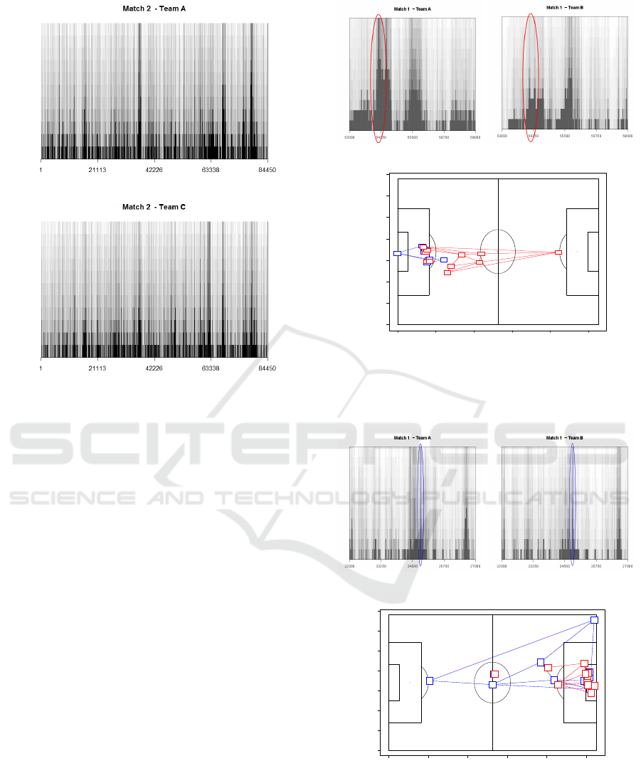
(a) Match 2 – Team A
(b) Match 2 – Team C
Figure 7: Graph visual rhythm images for teams of
Match 2.
55000 and 58000, we obtain the images shown in Fig-
ure 8. We plotted the corresponding graph from the
instant highlighted in red, to analyze the game strat-
egy employed in the time period related to a darker
block. It is possible to observe that for a darker block,
Team A (in blue) is compressed in a defensive strat-
egy while Team B (in red) is attacking. Team B is
well positioned in the field with many possibilities of
passes among players, which is represented in its own
graph visual rhythm image. Thus, entropy values may
represent team strategy both in attacking and defend-
ing perspectives. The distances among teammates de-
fine the team compactness on the pitch during attack-
ing and defending actions (Moura et al., 2012; Moura
et al., 2013). In this case, Team-A players occupy the
field in a very compact way, with a no clear purpose of
performing a man-to-man marking. This strategy may
favor the attacking team in order to allow a greater
number of options for passes between players. If this
condition is maintained over time (which is easily de-
tected in the graph visual rhythm image), it may in-
dicate a technical and tactical superiority for the team
with lower entropy values.
One goal was scored by Team A of Match 1 at
frame 24825. Figure 9 shows the graph visual rhythm
images associated with this moment. It is interesting
to notice that Team A was attacking, but, differently
from the situation depicted in Figure 8, both teams
(a) (b)
0 20 40 60 80 100
0 10 20 30 40 50 60 70
x
y
1
2
3
4
5
6
7
8
9
10
11
15
16
17
18
19
20
21
22
23
24
25
(c)
Figure 8: Graph Visual Rhythm in details: Highlighted dark
block and the corresponding match situation. Team A (in
blue) is compressed in a defensive strategy while Team B
(in red) is attacking.
(a) (b)
0 20 40 60 80 100
0 10 20 30 40 50 60 70
x
y
Graph Plot − Frame: 24825
1
2
3
4
5
6
7
8
9
10
11
15
16
17
18
19
20
21
22
23
24
25
1
2
3
4
5
6
7
8
9
10
11
15
16
17
18
19
20
21
22
23
24
25
(c)
Figure 9: Graph visual rhythms of teams at a goal event
timestamp.
have higher diversity entropy scores. In this case, this
phenomenon is observed due to the fact that the goal
was originated from a corner kick.
Visualizing Temporal Graphs using Visual Rhythms - A Case Study in Soccer Match Analysis
101

5.2 Most Valued Player: A
Centrality-oriented Perspective
We conducted a preliminary study considering the
computation of the betweeness centrality applied to
instant graphs. The intention here is to support the
identification of players whose centrality scores are
higher during the match, and so they could be con-
sidered more valued than others in the game strat-
egy. Figure 10 shows the centrality-based graph vi-
sual rhythm image for Match 2, using darker colors to
highlight players with higher centrality scores. It can
be noticed that during almost all the match, centrality
scores are low for most of the players. The low and
homogeneous centrality scores show that there was no
‘star topology.’ Each had nearly the same connectiv-
ity, indicating that the teams did not depend on one
single player (Clemente et al., 2015).
We can also notice that for Player 7 of Team A,
there were darker pixels along the match. By analyz-
ing his performance during the game, we could realize
that this player was involved in more passes than all
the others (47 passes in the first half time, while the
team’s passes average was 33.1), which could mean
that he was well positioned in the pitch during ball
possession.
This same pattern is observed for Team B. It is
possible to observe a darker pixel line for Player 6,
who was also the one involved in more passes (42
passes in the first half time against the team’s passes
average of 26.4). We observed similar patterns for
other matches: players with higher centrality scores,
when compared to teammates, are involved more fre-
quently with successful passes. Thus, graph visual
rhythm images allow to identify players who had in-
fluential contributions in a specific match, and, ap-
plied during the entire tournament, they may help
coaches to identify the most important players. In
other words, it helps to answer in an objective man-
ner whether, for example, the most famous players
fulfilled the expectations placed on them (Duch et al.,
2010). However, in a collective evaluation, both en-
tropy and centrality may be interpreted with caution.
The work of (Grund, 2012) shown in 760 matches in
the English Premier League that high levels of inter-
action (i.e., passing rate) lead to increased team per-
formance. However, centralized interaction patterns
lead to decreased team performance. In fact, even in
a social context, teams with denser networks had a
tendency to perform better and remain more viable.
Furthermore, these variables, analyzed over the
match, may help also to identify who are the play-
ers more affected by fatigue. By decreasing the num-
ber of players involved, it is possible to allow some
(a) Match 2 – Team A
(b) Match 2 – Team C
Figure 10: Graph visual rhythm images based on the play-
ers’ centrality for Match 2. We highlighted in red the play-
ers with higher centrality scores.
players to rest actively. Moreover, it can characterise
teams’ attacking strategies. The direct play may in-
crease centrality among some players and involves a
lot of participation from forwards and strikers, for ex-
ample (Clemente et al., 2015).
5.3 Patterns of Passes
We also investigated the possibility of using graph
visual rhythms for analyzing patterns of passes. In
this case, we have employed graphs defined by Flow
Networks. From soccer matches, we computed the
Ball Possession Flow Networks, in which vertices are
players and edges are passes accomplished among
teammates while the team has the ball possession.
Considering the first half time from each analyzed
match, it is possible to construct N different flow net-
work graphs, considering all N time intervals in which
each team has the ball possession. We computed the
graph visual rhythm image for each team in a match.
This image contains all passes accomplished among
teammates in each ball possession flow network, i.e.,
in this case, F
G
t
computes the occurrences of passes
among players. Pixels representing an specific pass
performed in a network were colored according to the
location in the pitch where the ball passing occurred.
Figure 11 shows color patterns used. We divided
IVAPP 2017 - International Conference on Information Visualization Theory and Applications
102

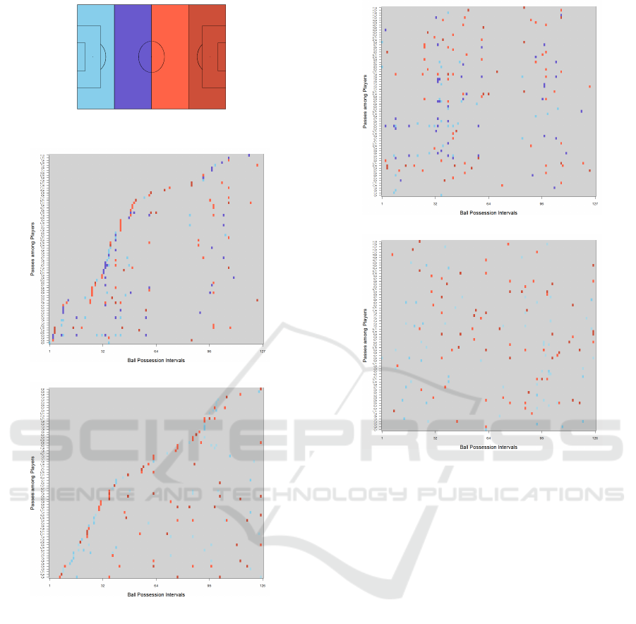
Figure 11: Pitch color patterns: defensive area in cold col-
ors, while attacking area in hot colors.
(a) Match 1 – Team A
(b) Match1 – Team B
Figure 12: Graph visual rhythms encoding the patterns of
passes of teams in Match 1.
the pitch in 4 sections, where defensive area of a team
was colored in cold colors (light blue and dark blue),
while attacking area of a team (the opponent’s pitch)
was colored in hot colors (light red and dark red).
Also, when a network does not have any edges (no
passes performed), all its pixels are grey. Using this
color pattern, it is possible to visually understand pat-
terns of passes for a team.
We analyzed the first half time of the same two
matches. The resulting graph visual rhythm images
are shown in Figures 12 and 14. The Y axis has labels
of players involved in successful passes (e.g., passes
from player 3 to player 10), and the X axis refers to
the flow networks considering ball possession. It is
(a) Match 1 – Team A
(b) Match1 – Team B
Figure 13: Graph visual rhythms (ordered by players) en-
coding the patterns of passes of teams in Match 1.
possible to notice some patterns in each match. Dur-
ing Match 1 (Figure 12), Team A performed more
passes among teammates than Team B (more colored
pixels in image of Team A). Also, Team A has longer
vertical lines of pixels colored, which means that for
each ball possession, many passes were activated in-
volving many players. Figure 13 presents a graph vi-
sual rhythm for this same match, but now with y-axis
representing passes ordered by players (from player 1
to 11). It is also possible to notice that many passes
(vertical pixel lines) involve both defensive, middle,
and forward players, in different field regions. Fur-
thermore, some passes occurred many times along
networks, and some of them only in its defensive area
(cold-colored pixels). Team B has performed less ball
passes, and passes in a single ball possession period
involve only two players. Most of those passes occur
in the attacking area (predominance of hot-colored
pixels).
During Match 2 (Figure 14), Team B has per-
formed more passes than Team A. It is interesting to
notice that many of them occurred in its defensive
area (predominance of cold-colored pixels), while
Visualizing Temporal Graphs using Visual Rhythms - A Case Study in Soccer Match Analysis
103

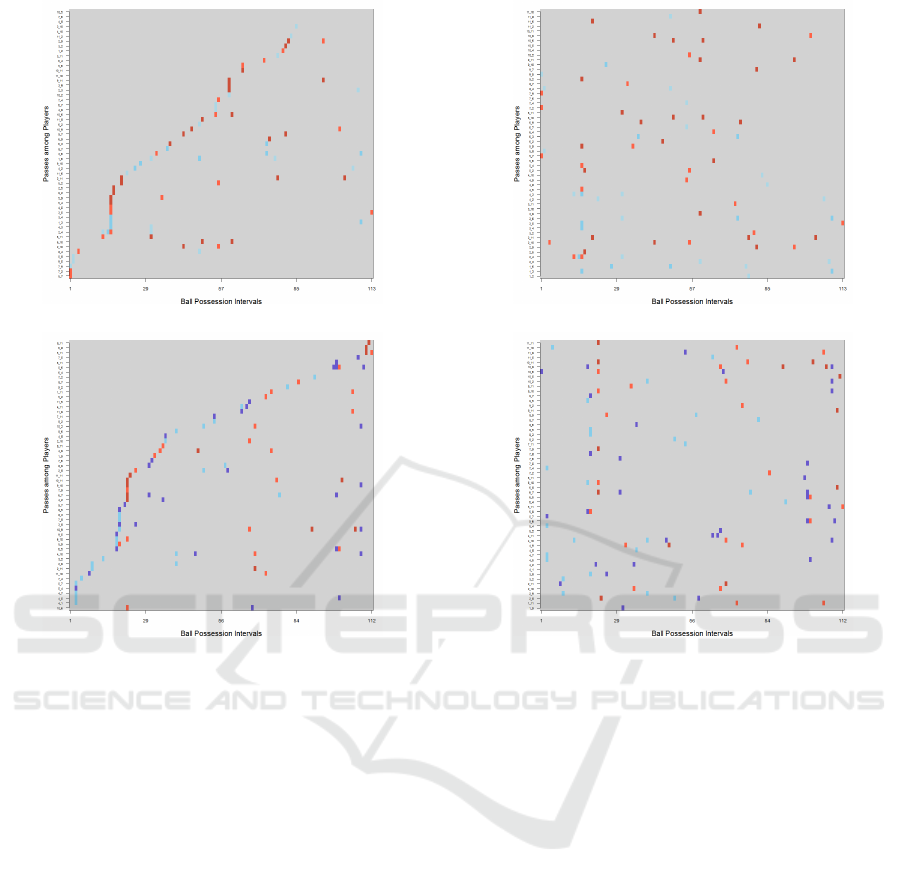
(a) Match 2 – Team A
(b) Match 2 – Team C
Figure 14: Graph visual rhythms encoding the patterns of
passes of teams in Match 2.
team A performs more passes in the attacking area.
Figure 15 presents a graph visual rhythm for this same
match, but now with y-axis representing passes or-
dered by players (from player 1 to 11). It can be
noticed that ball possession involves few players. In
this match, Team C performed passes involving more
players, from defensive to forward players. Note also
that for two different matches, Team A has very dif-
ferent performance in terms of patterns of passes (see
Figures 12(a) and 14(a)).
5.4 Pass Patterns in Attack Actions
It is also possible to create graph visual rhythm im-
ages considering a subset of players. For example,
it might be interesting to show pass patterns involv-
ing only forward players. With this purpose, we cre-
ated graph visual rhythms from passes involving only
players with role, which is depicted in Figure 16. In
this case, we refer to Match 1. We can observe that
not only did forward players of Team A accomplish
more passes than players of Team B, but also they
accomplished those passes in the opponent area (pre-
(a) Match 2 – Team A
(b) Match 2 – Team C
Figure 15: Graph visual rhythms (ordered by players) en-
coding the patterns of passes of teams in Match 2.
dominance of hot-colored pixels). We can conclude
that Team A exploited more frequently the strategy of
using multiple passes in attacking actions.
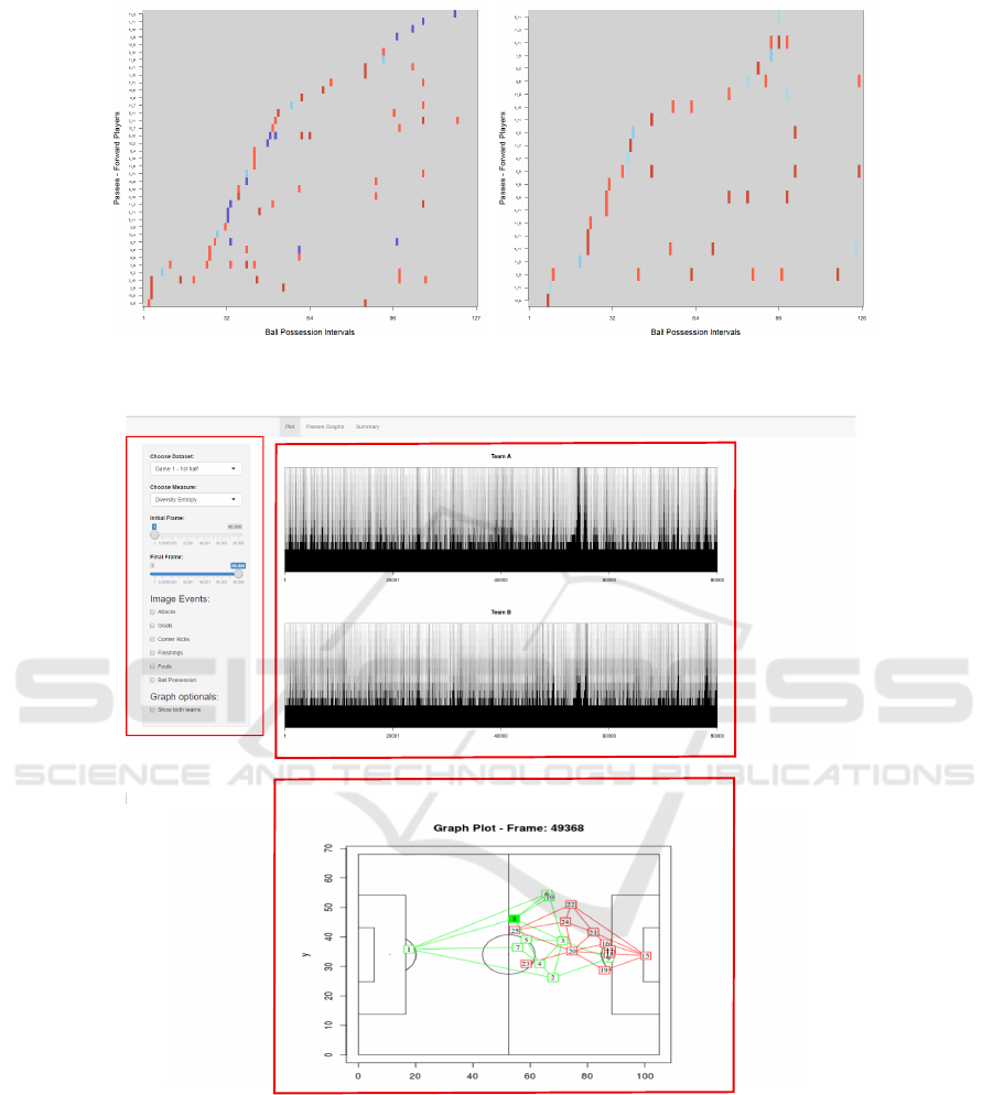
5.5 Soccer Visual Analytics Tool
We have created a soccer visual analytics tool that
integrates the different graph extraction approaches,
and visual rhythm image computation algorithms de-
scribed in this paper. This tool allows loading data
about soccer matches (usually, information about
players’ location over time), and encode them into
graphs, depending on the type of analysis defined by
the user. All complex network measures described in
this paper were implemented, so it is possible to visu-
ally analyze them by means of graph visual rhythms.
Figure 17 presents a typical usage example. In
this case, we have graph visual rhythm images of two
teams computed from instant graphs represented by
the diversity entropy of their vertices. By clicking
on the side-bar check boxes (area labeled with A), a
user can highlight match events, as goals and attack-
ing moments, and also, can define a specific period of
IVAPP 2017 - International Conference on Information Visualization Theory and Applications
104

(a) (b)
Figure 16: Graph visual rhythms encoding the patterns of passes of forward players in Match 1.
A
B
C
Figure 17: Screen shot of the soccer visual analytics tool developed.
time for zooming in targeting specific regions of the
images (shown in region B). User can also view corre-
sponding graphs or temporal graphs videos, by click-
ing anywhere on the graph visual rhythm image, or
selecting an area of interest in the image (field graph
view in region C).
6 CONCLUSIONS
This paper has introduced the graph visual rhythm
representation, a compact visual structure to encode
changes in temporal graphs, making it a suitable so-
lution to handle large volumes of data. We demon-
strate its applicability in several usage scenarios con-
cerning the analysis of soccer matches, whose several
Visualizing Temporal Graphs using Visual Rhythms - A Case Study in Soccer Match Analysis
105

dynamic aspects are encoded into temporal graphs.
This research opens novel opportunities for inves-
tigation related to the use of several image process-
ing algorithms to highlight important patterns in tem-
poral graphs. We plan to follow this research venue
in our future work. We also plan to incorporate ma-
trix reordering methods (Behrisch et al., 2016) aim-
ing to improve the identification of changing patterns
in graph visual rhythm representations. Another is-
sue refers to the implementation of suitable visualiza-
tion approaches to handle players’ substitutions in a
match.
ACKNOWLEDGEMENTS
The authors would like to thank CAPES, CNPq (grant
#306580/2012-8), FAPESP (grants #2013/50169-1
and #2013/50155-0 ) for the financial support. Au-
thors are also grateful for the support of PUC-
Campinas.
REFERENCES
Bach, B., Pietriga, E., and Fekete, J. (2014). Visualiz-
ing dynamic networks with matrix cubes. In CHI
Conference on Human Factors in Computing Systems,
CHI’14, Toronto, ON, Canada - April 26 - May 01,
2014, pages 877–886.
Beck, F., Burch, M., Diehl, S., and Weiskopf, D. (2016). A
taxonomy and survey of dynamic graph visualization.
Computer Graphics Forum.
Behrisch, M., Bach, B., Riche, N. H., Schreck, T., and
Fekete, J. (2016). Matrix reordering methods for table
and network visualization. Comput. Graph. Forum,
35(3):693–716.
Bezerra, F. N. and Lima, E. (2006). Low cost soccer video
summaries based on visual rhythm. In Proceedings of
the 8th ACM SIGMM International Workshop on Mul-
timedia Information Retrieval, MIR 2006, October 26-
27, 2006, Santa Barbara, California, USA, pages 71–
78.
Brandes, U. and Corman, S. R. (2003). Visual Unrolling
of Network Evolution and the Analysis of Dynamic
Discourse. Information Visualization, 2(1):40–50.
Brandes, U., Indlekofer, N., and Mader, M. (2012). Visual-
ization methods for longitudinal social networks and
stochastic actor-oriented modeling. Social Networks,
34(3):291–308.
Burch, M., H
¨
oferlin, M., and Weiskopf, D. (2011). Layered
timeradartrees. In 15th International Conference on
Information Visualisation, IV 2011, London, United
Kingdom, July 13-15, 2011, pages 18–25.
Casteigts, A., Flocchini, P., Quattrociocchi, W., and San-
toro, N. (2011). Time-Varying Graphs and Dynamic
Networks Ad-hoc, Mobile, and Wireless Networks.
6811(5):346–359.
Chun, S. S., Kim, H., Kim, J., Oh, S., and Sull, S. (2002).
Fast text caption localization on video using visual
rhythm. In Recent Advances in Visual Information
Systems, 5th International Conference, VISUAL 2002
Hsin Chu, Taiwan, March 11-13, 2002, Proceedings,
pages 259–268.
Clemente, F., Couceiro, M., Martins, F., and Mendes, R.
(2015). Using network metrics in soccer: A macro-
analysis. J Sports Sci., 45:123134.
Costa, L. d. F., Rodrigues, F. A., Travieso, G., and Vil-
las Boas, P. R. (2007). Characterization of complex
networks: A survey of measurements. Advances in
physics, 56(1):167–242.
Cotta, C., Mora, A. M., Merelo, J. J., and Merelo-Molina,
C. (2013). A network analysis of the 2010 fifa world
cup champion team play. Journal of Systems Science
and Complexity, 26(1):21–42.
da Silva Pinto, A., Schwartz, W. R., Pedrini, H., and
de Rezende Rocha, A. (2015). Using visual
rhythms for detecting video-based facial spoof at-
tacks. IEEE Trans. Information Forensics and Secu-
rity, 10(5):1025–1038.
Duch, J., Waitzman, J. S., and Amaral, L. a. N. (2010).
Quantifying the performance of individual players in
a team activity. PloS one, 5(6):e10937.
Figueroa, P. J., Leite, N. J., and Barros, R. M. L. (2006a).
Background recovering in outdoor image sequences:
An example of soccer players segmentation. Image
Vision Comput., 24(4):363–374.
Figueroa, P. J., Leite, N. J., and Barros, R. M. L. (2006b).
Tracking soccer players aiming their kinematical mo-
tion analysis. Computer Vision and Image Under-
standing, 101(2):122–135.
Grund, T. (2012). Network structure and team performance:
The case of english premier league soccer teams. So-
cial Networks, 34(4):682–690.
Guimar
˜
aes, S. J. F., Couprie, M., de Albuquerque Ara
´
ujo,
A., and Leite, N. J. (2003). Video segmentation based
on 2d image analysis. Pattern Recognition Letters,
24(7):947–957.
Hurter, C., Ersoy, O., Fabrikant, S. I., Klein, T. R., and
Telea, A. C. (2014). Bundled visualization of dynamic
graph and trail data. IEEE Transactions on Visualiza-
tion and Computer Graphics, 20(8):1141–1157.
Leskovec, J., Kleinberg, J., and Faloutsos, C. (2005).
Graphs over Time: Densification Laws, Shrinking Di-
ameters and Possible Explanations. In KDD, pages
177–187.
Moura, F. A., Martins, L. E., and Cunha, S. E. (2014). Anal-
ysis of football game-related statistics using multivari-
ate techniques. J Sports Sci., 32(20):1881–1887.
Moura, F. A., Martins, L. E. B., Anido, R. D. O., Barros,
R. M. L. D., and Cunha, S. A. (2012). Quantitative
analysis of brazilian football players’ organisation on
the pitch. Sports Biomechanics, 11(1):85–96. PMID:
22518947.
Moura, F. A., Martins, L. E. B., Anido, R. O., Ruffino, P.
R. C., Barros, R. M. L., and Cunha, S. A. (2013).
IVAPP 2017 - International Conference on Information Visualization Theory and Applications
106

A spectral analysis of team dynamics and tactics
in Brazilian football. Journal of sports sciences,
31(14):1568–77.
Nahman, J. and Peri, D. (2017). Path-set based optimal
planning of new urban distribution networks. Interna-
tional Journal of Electrical Power & Energy Systems,
85:42 – 49.
Ngo, C., Pong, T., and Chin, R. T. (1999). Detection
of gradual transitions through temporal slice analy-
sis. In 1999 Conference on Computer Vision and Pat-
tern Recognition (CVPR ’99), 23-25 June 1999, Ft.
Collins, CO, USA, pages 1036–1041.
Passos, P., Davids, K., Araujo, D., Paz, N., Mingu
´
ens, J.,
and Mendes, J. (2011). Networks as a novel tool for
studying team ball sports as complex social systems.
Journal of Science and Medicine in Sport, 14(2):170–
176.
Pe
˜
na, J. L. and Touchette, H. (2012). A network the-
ory analysis of football strategies. arXiv preprint
arXiv:1206.6904.
Preparata, F. P. and Shamos, M. (2012). Computational ge-
ometry: an introduction. Springer Science & Business
Media.
Santoro, N., Quattrociocchi, W., Flocchini, P., Casteigts, A.,
and Amblard, F. (2011). Time-Varying Graphs and
Social Network Analysis: Temporal Indicators and
Metrics.
Travenc¸olo, B. A. N. and Costa, L. d. F. (2008). Ac-
cessibility in complex networks. Physics Letters A,
373(1):89–95.
Travenc¸olo, B. A. N., Viana, M. P., and Costa, L. D. F.
(2009). Border detection in complex networks. New
Journal of Physics, 11.
Vehlow, C., Burch, M., Schmauder, H., and Weiskopf, D.
(2013). Radial layered matrix visualization of dy-
namic graphs. In 17th International Conference on
Information Visualisation, IV 2013, London, United
Kingdom, July 16-18, 2013, pages 51–58.
Zhao, F. and Tung, A. K. H. (2012). Large scale cohesive
subgraphs discovery for social network visual analy-
sis. PVLDB, 6(2):85–96.
Visualizing Temporal Graphs using Visual Rhythms - A Case Study in Soccer Match Analysis
107