
Frequency Domain Analysis of Acoustic Emission Signals in Medical
Drill Wear Monitoring
Zrinka Murat
1
, Danko Brezak
1
, Goran Augustin
2
and Dubravko Majetic
1
1
Faculty of Mechanical Engineering and Naval Architecture, University of Zagreb, Ivana Lucica 5, Zagreb, Croatia
2
University Hospital Center Zagreb and School of Medicine, University of Zagreb, Kispaticeva 12, Zagreb, Croatia
Keywords: Bone Drilling, Drill Wear, Acoustic Emission, Neural Networks, Data Mining.
Abstract: Medical drills are subject to wear process due to mechanical, thermal and, potentially, sterilisation
influences. The influence of drill wear on friction contributes to the drilling temperature rise and occurrence
of thermal osteonecrosis. During the cutting process drilling temperature cannot be adequately reduced by
applying cooling fluid externally on the bone surface and a part of a tool which is not in the contact with the
bone if higher wear rates occurs. Since it is not possible to directly establish or measure drill wear rate
without interrupting the machining process, this important parameter should be estimated using available
process signals. Therefore, the application of tool wear features extracted from acoustic emission signals in
the frequency domain for the purpose of indirect medical drill wear monitoring process has been studied in
detail and the results are presented in this paper.
1 INTRODUCTION
Beside several important factors related to the drill
design, machining parameters, drilling depth, and
cooling technique, drill wear rate is one of the most
influential factors in temperature increase during
bone drilling and potential occurrence of thermal
osteonecrosis. Medical drills wear out due to the
mechanical, and potentially also chemical and
thermal factors which occur during sterilization and
continuous application in different cutting
conditions. Higher wear rate induces higher friction
in the cutting zone, and consequently higher forces
and heat generation. This logical and a well-known
relationship has been confirmed several decades ago
by Mathews and Hirsch, 1972, when they compared
new drills with the used one which drilled more than
200 holes. As expected, worn drills caused higher
temperatures during drilling.
Importance of a drill wear rate on bone thermal
damages has been also emphasised in the more
recent study performed by Allan, Williams, and
Kerawala, 2005, where three types of drills were
compared: new one, drill which drilled 600 holes,
and drill which were used for several months. The
results have shown important differences in mean
temperature rise values – from 7.5
o
C (unworn drill)
to 25.4
o
C (completely worn drill), measured in
relation to the initial bone temperature of 37
o
C.
Authors suggested drill replacement after every
surgical intervention.
The same negative influence of drill wear has
been reported in Chacon et al., 2006, Querioz et al.,
2008, and Jochum and Reichart, 2000, where the
temperature rise and thermal osteonecrosis is noticed
after only 25, 30 and 40 drilled holes, respectively.
According to the Singh, Davenport and Pegg,
2010, whose research included 40 hospitals in the
Great Britain, 75% of them had no guidelines for
controlling and maintenance of medical drills. The
remaining 10 hospitals confirmed they have
instructions related to the identification and labelling
of worn drills, and 8 of them confirmed that they
actually implemented those regulations. From the
total number of hospitals, 45% of them said that they
use single-used medical drills. At the end of their
report authors point to the frequent application of
worn drills, as well as the absence of any consensus
regarding the tool wear inspection.
Although there has been many papers published
in the past 25 years considering tool wear
monitoring and identification in industrial
applications (Jantunen, 2002), comprehensive
analyses in the field of medical drilling are still
missing. Industrial drilling dynamics usually differ
from the one in medical applications in view of
Murat Z., Brezak D., Augustin G. and Majetic D.
Frequency Domain Analysis of Acoustic Emission Signals in Medical Drill Wear Monitoring.
DOI: 10.5220/0006150401730177
In Proceedings of the 10th International Joint Conference on Biomedical Engineering Systems and Technologies (BIOSTEC 2017), pages 173-177
ISBN: 978-989-758-212-7
Copyright
c
2017 by SCITEPRESS – Science and Technology Publications, Lda. All rights reserved
173
different drill characteristics, machining parameters,
and workpiece material characteristics. Therefore, it
is necessary to establish the possibility of applying
some of the proposed industrial solutions to medical
drill wear monitoring. First analyses have confirmed
the applicability of multi-sensor concept and
advanced decision algorithms in the on-line medical
drill wear monitoring (Staroveski et al., 2014,
Staroveski, Brezak and Udiljak, 2015).
In one of those two studies (Staroveski, Brezak
and Udiljak, 2015) two types of signals were
analysed: servomotor currents and acoustic
emission. The acoustic emission signals were
roughly processed in a way that each signal was
fragmented in the frequency domain into 7 samples
(between 50-400 kHz). Each sample was related to
the belonging 50 kHz frequency bandwidth (50-100,
100-150;...; 350-400 kHz). Drill wear features were
then extracted from every sample individually. Since
there was only one, arbitrarily chosen bandwidth (50
kHz), additional analysis with different frequency
bandwidths has been performed in this study in
order to determine the full potential of AE signals in
surgical drill wear monitoring.
The paper is organised as follows. Section 2
describes experimental setup and parameters used in
data acquisition process, while Section 3 explains a
method for drill wear feature extraction from
measured AE signals. In Section 4 neural network
classifier algorithm is briefly presented, and Section
5 includes drill wear rate classification results.
Concluding remarks are finally summarised in
Section 6.
2 EXPERIMENTAL DETAILS
Acoustic emission (AE) signals have been measured
during bone drilling on the 3-axis bench-top mini
milling machine adjusted for the purpose of this
research (Figure 1). The machine has been
retrofitted with the 0.4 kW (1.27 Nm) permanent
magnet synchronous motors with integrated
incremental encoders (type Mecapion SB04A),
corresponding motor controllers (DPCANIE-
030A400 and DPCANIE-060A400), ball screw
assemblies, and LinuxCNC open architecture control
(OAC) system. AE signals were measured using
Kistler piezoelectric industrial accelerometer type
8152B1 coupled with 5125B interface module. The
sensor was mounted on the flange used to attach
main spindle motor to Z-axis, near the motor front
bearing and the drill. Its measuring range was from
50 to 400 kHz.
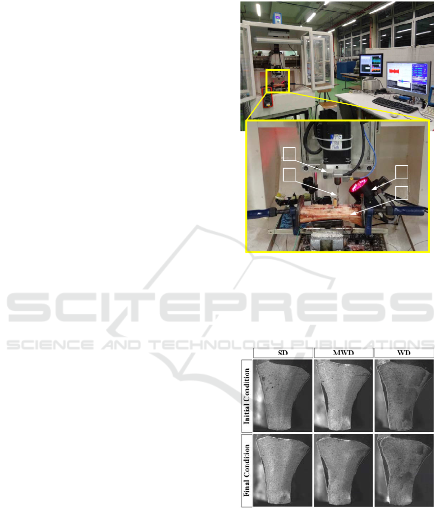
1) Acoustic emission sensor
2) Medical drill
3) Industrial CCD camera with telecentric
lens system
4) Bovine bone specimen
4
2
1
3
Figure 1: Experimental setup.
Figure 2: Images of cutting edges at the beginning and at
the end of the drilling experiment with the sharp drill
(SD), medium worn drill (MWD) and worn drill (WD).
Drill wear is observable as a dark area along the cutting
edge on the drill flank.
Three types of standard, 4.5 mm in diameter,
medical drills (Komet Medical Gmbh, S2727.098)
with two flutes and a point angle of 90
o
were used in
BIOSIGNALS 2017 - 10th International Conference on Bio-inspired Systems and Signal Processing
174

the experiment. They only differed in the amount of
drill flank wear level (Figure 2). First type belonged
to a group of sharp drill (SD), second type was
categorised as a medium worn drill (MD), and third
type was defined as a worn drill (WD). Drilling
temperature for WD type of a drill exceeded 55
o
C in
almost all measured samples.
Three cutting speed values were combined with
four different feed rates (Table 1), and for each of
those twelve combinations of machining parameters
ten measurements were performed using randomly
selected approach (two consecutive measurements
had different machining parameters). Altogether,
360 sets of data (120 sets for each drill wear level -
SD, MWD, WD) have been recorded.
Table 1: Combinations of machining parameters.
Cutting speed (v
c
),
Rotational speed
*
Feed rate (f)
mm/rev
0.01 0.03 0.05 0.1
m/min rev/min
*
mm/s
10 707.4 0.12 0.35 0.59 1.18
30 2122.1 0.35 1.06 1.77 3.54
50 3536.8 0.59 1.77 2.95 5.90
Bone specimens were prepared using fresh
bovine tibia with average diaphysis cortical
thickness (drilling depth) of 8.5 mm and variable
mechanical properties (hardness). AE signal sample
was taken during one cortical bone drilling layer,
and when drill entered into cancellous bone it was
removed from the hole, moved along Y-axis for
5 mm and positioned for the next drilling operation.
3 DRILL WEAR FEATURES
EXTRACTION
Samples of AE signals were taken using multi-
function high-speed data acquisition I/O board PCI-
DAS4020/12. For every hole, signals were measured
for 0.1 second with the sampling rate of 2 MHz after
both cutting edges completely entered into the
cortical bone. Measured AE signals were then
analysed in the frequency domain using Fast Fourier
transform (FFT) method. Analyses were performed
within the AE sensor measuring range (50-400 kHz).
Each signal has been divided into a series of
samples depending on a chosen frequency
bandwidth, and for each sample power spectrum
density (PSD) was established. Since in Staroveski,
Brezak and Udiljak, 2015, a 50 kHz frequency
bandwidth was used, six additional and different
bandwidths (5, 10, 15, 20, 30, and 40 kHz) were
analysed in this study. In another words, in the case
of 5 kHz bandwidth we got 70 samples per signal
(each sample related to 70 different bandwidths
within the 50-400kHz interval), while for 40 kHz
bandwidth signal was divided into 9 samples, i.e.,
50-90 kHz, 90-130 kHz, ...., 330-370kHz, and 370-
400 kHz (the last sample had 30 kHz bandwidth
because the upper frequency value cannot exceed
sensor measurement range of 400 kHz).
Energy of each sample of the analysed AE signal
has been calculated from the expression
2
U
L
f
y
f
Sdf,
(1)
where S
y
is one-sided PSD function of the AE signal,
while f
L
and f
U
are lower and upper frequency values
chosen to reflect the energy in the range of interest
(Scheffer, Heyns and Klocke, 2003).
Energy values of all samples of AE signals were
used together with the belonging combination of
feed rate and cutting speed as drill wear features in
the classification of one of three analysed drill wear
conditions (SD, MWD, WD).
4 NEURAL NETWORK
CLASSIFIER
Drill wear level classification was performed by
using a well-known three-layered feed-forward
Radial Basis Function Neural Network (RBFNN).
This type of a neural network has good classification
capabilities and can be trained in one step with
simple hidden layer structure adaptation in view of
the learning problem.
In the training phase matrix of synaptic weights c
is calculated from the expression:
1
,cHy
(2)
where y stands for the matrix of desired output
values and H is the matrix of hidden layer neurons
(RBF activation functions) outputs. Since Gauss
function was used as an activation function in this
study, elements of matrix H are determined using
the expression:
xt
2
ij
2
j
ij
exp
H
= , i=1, ..., N, j=1, ..., K,
(3)
where x
i
is a vector composed from ith element of
all (L) input vectors, t
j
is a jth hidden layer neuron
Frequency Domain Analysis of Acoustic Emission Signals in Medical Drill Wear Monitoring
175

position center vector, and
j
is an activation or
RBF function width of the jth hidden layer neuron.
Gaussian widths are calculated as a geometrical
mean value of the Euclidean distances of the centre
of the jth neuron and the centers of two of his
neighbor neurons:
12
jjj
=pp,
(4)
where p
1j
is the Euclidean distance between the jth
neuron centre and the (j-1)th neuron centre, and p
2j
is the Euclidean distance between the jth neuron
centre and the (j+1)th neuron centre.
Matrix H was quadratic matrix in this study,
since the number of hidden layer neurons was equal
to the number of data set samples used in the
training phase (K = N).
In the testing phase, matrix or, in this case, three-
element vector of desired output values y is obtained
from the expression:
Hcy
.
(5)
Before entering in the training phase, all
classifier input data values were normalised in the
interval (0, 1). Elements of vector y or classifier
outputs were defined as either "0" or "1", depending
on the drill wear level class to which analysed
combination of input features belonged to (network
output belonging to the actual class was defined as
"1" and the remaining two outputs as "0").
5 RESULTS AND ANALYSIS
For every combination of RBFNN inputs, 360 data
sets have been prepared. They were then divided
into two groups, where 180 sets were used in the
RBFNN classifier training phase, and the remaining
180 in its testing phase. Data used in the testing
phase were additionally divided into 5 groups or
tests (T1 – T5). Each group was composed from 36
samples belonging to each of 36 different
combinations of machining parameters and drill
wear levels (three cutting speed values combined
with four different feed rates and three drill wear
levels).
Performance analysis of drill wear features has
been carried out in two steps. At first, energy values
belonging to every analysed frequency bandwidth of
the AE signals were individually analysed in
combination with machining parameters using
RBFNN classifier. Results were compared using
performance index defined as Classification Success
Rate (CSR), i.e., the ratio of successfully classified
samples to all tested samples.
All those features which satisfied minimal
predefined CSR value (CSR_min) were taken in the
second phase of the analysis. Based on the CSR
values obtained for all drill wear features
individually, two CSR limits have been established:
CSR_min = 50% and CRS_min = 60%.
In the second phase of this analysis, features that
satisfied abovementioned conditions were mutually
combined and tested again. Classification success
rates of those combinations are presented in Tables
2, 3, and 4. Features were first combined for each
analysed frequency bandwidth separately (Table 2
and 3) and then additionally regardless to the
bandwidth association (Table 4).
Table 2: Classification success rates of tests composed of
all drill wear features (AE signal energies) of the analysed
frequency bandwidth that individually fulfilled condition
CSR_min ≥ 50%.
Frequency
b
andwidth,
kHz
CSR of the tests, %
T1 T2 T3 T4 T5 Avg.
5
97.2 97.2 94.4 100 94.4 96.6
10
94.4 94.4 86.1 97.2 97.2 93.9
15
94.4 88.9 97.2 97.2 94.4 94.4
20
94.4 97.2 88.9 94.4 97.2 94.4
100 97.2 94.4 91.7 94.4 95.6
40
91.7 91.7 86.1 91.7 94.4 91.1
Table 3: Classification success rates of tests composed of
all drill wear features (AE signal energies) of the analysed
frequency bandwidth that individually fulfilled condition
CSR_min ≥ 60%.
Frequency
b
andwidth,
kHz
CSR of the tests, %
T1 T2 T3 T4 T5 Avg.
5
91.7 88.9 100 97.2 94.4 94.4
10
94.4 97.2 88.9 97.2 100 95.6
15
97.2 97.2 94.4 94.4 100 96.7
20
94.4 88.9 100 88.9 91.7 92.8
30
97.2 94.4 97.2 94.4 91.7 95.0
40
91.7 83.3 91.7 77.8 83.3 85.6
Table 4: Classification success rates of tests composed of
all drill wear features (AE signal energies) of all analysed
frequency bandwidths that individually fulfilled condition
CSR_min ≥ 50% and CSR_min ≥ 60%.
CSR_min,
%
CSR of the tests, %
T1 T2 T3 T4 T5 Avg.
50
97.2 97.2 91.7 91.7 97.2 95.0
60
86.1 88.9 94.4 91.7 97.2 91.7
Practically all combinations of energy features
BIOSIGNALS 2017 - 10th International Conference on Bio-inspired Systems and Signal Processing
176

related to each frequency bandwidth separately
accomplished high classification success rate of
more than 90% (Table 2 and 3). However, if the
results from Table 2 (CSR_min = 50%) are
compared with the one presented in Staroveski,
Brezak and Udiljak, 2015, (Table 5) where
frequency bandwidth was 50 kHz, a slight
improvement in classifier accuracy can be observed,
particularly in the case of the features extracted from
the samples with narrowest bandwidth of 5 kHz.
Table 5: Classification success rates of tests composed of
all drill wear features (AE signal energies) of the 50 kHz
frequency bandwidth that individually fulfilled condition
CSR_min ≥ 50% (Staroveski, Brezak and Udiljak, 2015).
Frequency
bandwidth,
kHz
CSR of the tests, %
T1 T2 T3 T4 T5 Avg.
50 86.1 91.7 94.4 86.1 91.7 90
Combination of energy features from different
frequency bandwidths (Table 4) obtained very
similar results to those presented in Table 2 and 3.
6 CONCLUSIONS
Analysis of medical drill wear features extracted
from the AE signals in the frequency domain using
different frequency bandwidths has been presented
in this study. Features were used to identify one of
the three drill wear levels. Application of the AE
signals in medical drill wear monitoring can be very
useful due to the fact that that type of the signal has
already shown insensitivity to variations of bone
mechanical properties. This study has additionally
confirmed high precision of the AE signals in drill
wear level classification from sharp to completely
worn drill. Although only slight improvement has
been observed in comparison with the results from
one of the previous study (around 6% higher
classification precision), it can nevertheless
positively contribute to the design of a reliable and
precise multi-sensor medical drill wear estimators.
Their purpose would be to reduce mechanical and
thermal bone damages in the case of fully automated
next-generation bone drilling machines applications.
ACKNOWLEDGEMENTS
This work has been fully supported by the Croatian
Science Foundation under the project number IP-09-
2014-9870.
REFERENCES
L. S. Mathews, C. Hirsch, 1972, Temperature measured in
human cortical bone when drilling, The Journal of
Bone Joint Surgery, 54-A, pp. 297-308.
W. Allan, E. D. Williams, C. J. Kerawala, 2005, Effects of
repeated drill use on temperature of bone during
preparation for osteosynthesis self-tapping screws,
British Journal of Oral and Maxillofacial Surgery, 43,
pp. 314-319.
G. E. Chacon, D. L. Bower, P. E. Larsen, E. A.
McGlumphy, F.M. Beck, 2006, Heat Production by 3
Implant Drill Systems After Repeated Drilling and
Sterilization, Journal of Oral and Maxillofacial
Surgery, 64, pp. 265-269.
T. P. Queiroz, F. Á. Souza, R. Okamoto, R. Margonar, V.
A. Pereira-Filho, I. R. Garcia, E. H. Vieira, 2008,
Evaluation of Immediate Bone-Cell Viability and of
Drill Wear After Implant Osteotomies:
Immunohistochemistry and Scanning Electron
Microscopy Analysis, Journal of Oral and
Maxillofacial Surgery, 66, pp. 1233-1240.
R. M. Jochum, P. A. Reichart, 2000, Influence of multiple
use of Timedur® – titanium cannon drills: thermal
response and scanning electron microscopic findings,
Clinical Oral Implants Research, 11, pp. 139-143.
J. Singh, J. H. Davenport, D. J. Pegg, 2010, A national
survey of instrument sharpening guidelines, The
Surgeon, 8, pp. 136-139.
E. Jantunen, A summary of methods applied to tool
condition monitoring in drilling, 2002, International
Journal of Machine Tools & Manufacture, 42, pp. 997-
1010.
T. Staroveski, D. Brezak, V. Grdan, T. Bacek, 2014,
Medical Drill Wear Classification Using Servomotor
Drive Signals and Neural Networks, Lecture Notes in
Engineering and Computer Science, 2211 (1), pp. 599-
603.
T. Staroveski, D. Brezak, T. Udiljak, 2015, Drill wear
monitoring in cortical bone drilling, Medical
engineering & physics, 37 (6), pp. 560-566.
C. Scheffer, P. S. Heyns, F. Klocke, 2003, Development of
a tool wear-monitoring system for hard turning,
International Journal of Machine Tools and
Manufacturing,43, pp.973–85.
Frequency Domain Analysis of Acoustic Emission Signals in Medical Drill Wear Monitoring
177
