
Statistical Analysis of Window Sizes and Sampling Rates in Human
Activity Recognition
Anzah H. Niazi
1
, Delaram Yazdansepas
2
, Jennifer L. Gay
3
, Frederick W. Maier
1
,
Lakshmish Ramaswamy
2
, Khaled Rasheed
1,2
and Matthew P. Buman
4
1
Institute for Artificial Intelligence, The University of Georgia, Athens, Georgia, U.S.A.
2
Department of Computer Science, The University of Georgia, Athens, Georgia, U.S.A.
3
College of Public Health, The University of Georgia, Athens, Georgia, U.S.A.
4
School of Nutrition and Health Promotion, Arizona State University, Phoenix, Arizona, U.S.A.
Keywords:
Actigraph g3x+, Analysis of Variance, Body-worn Accelerometers, Data Mining, Human Activity Recogni-
tion, Random Forests, Sampling Rate, Weighted Least Squares, WEKA, Window Size.
Abstract:
Accelerometers are the most common device for data collection in the field of Human Activity Recognition
(HAR). This data is recorded at a particular sampling rate and then usually separated into time windows be-
fore classification takes place. Though the sampling rate and window size can have a significant impact on the
accuracy of the trained classifier, there has been relatively little research on their role in activity recognition.
This paper presents a statistical analysis on the effect the sampling rate and window sizes on HAR data classi-
fication. The raw data used in the analysis was collected from a hip-worn Actigraphy G3X+ at 100Hz from 77
subjects performing 23 different activities. It was then re-sampled and divided into windows of varying sizes
and trained using a single data classifier. A weighted least squares linear regression model was developed and
two-way factorial ANOVA was used to analyze the effects of sampling rate and window size for different ac-
tivity types and demographic categories. Based upon this analysis, we find that 10-second windows recorded
at 50Hz perform statistically better than other combinations of window size and sampling rate.
1 INTRODUCTION
The field of Human Activity Recognition (HAR) is
dependent on a variety of instruments for data col-
lection — heart rate monitors, GPS, light sensors,
etc. — of which wearable triaxial accelerometers
are the most commonly utilized (Lara and Labrador,
2013), (Preece et al., 2009). Accelerometers are com-
mercially available in many formats, from modern
smartphones and consumer-grade activity-monitoring
products to high-grade research-oriented devices, the
consequences of which are wide degrees of quality in
data collection for HAR. When preparing for data col-
lection in a HAR study, two aspects of the accelerom-
eter to use should be strongly considered: the place-
ment of the device and the sampling rate at which it
gathers data.
The placement of the device depends greatly on
the context of the study. Many studies focusing on
ambulation activities (walking, running etc.) prefer
hip-worn or wrist-worn devices (Lara and Labrador,
2013), both of which have advantages and disadvan-
tages. Wrist-worn devices have trouble distinguishing
lower-body activities (for instance, walking and stair
climbing), while hip-worn devices can be problematic
when recognizing upper-body activities (for instance,
eating and brushing teeth). The impact of sampling
rate is discussed in later sections.
Once data has been collected — typically at a
fixed sampling rate — it is prepared for classifica-
tion by extracting relevant features such as means
and standard deviations and dividing the accelerom-
eter readings into windows. Often, windows of fixed
length are used.
Both the sampling rate and window size of data
are crucial decisions in HAR which directly affect the
accuracy of developed classifiers. Though a literature
review revealed some relevant analyses (Section 2),
there appears to be a relative dearth of work directly
addressing sampling rate and window size in HAR.
This study is an attempt to remedy what we perceive
as a gap in the research. We have attempted to statisti-
cally identify the window size and sampling rate com-
bination which best suits activity recognition across
demographical and activity divisions.
The data used in this study was obtained from
77 demographically diverse subjects for 23 activities
in studies performed at Arizona State University in
Niazi A., Yazdansepas D., Gay J., Maier F., Ramaswamy L., Rasheed K. and Buman M.
Statistical Analysis of Window Sizes and Sampling Rates in Human Activity Recognition.
DOI: 10.5220/0006148503190325
In Proceedings of the 10th International Joint Conference on Biomedical Engineering Systems and Technologies (BIOSTEC 2017), pages 319-325
ISBN: 978-989-758-213-4
Copyright
c
2017 by SCITEPRESS – Science and Technology Publications, Lda. All rights reserved
319

Table 1: Description of Activities Performed.
# Activity Duration or Distance # of
sub-
jects
1 Treadmill at 27 młmin-1 (1mph) @ 0% grade 3 min 29
2 Treadmill at 54 młmin-1 (2mph) @ 0% grade 3 min 21
3 Treadmill at 80 młmin-1 (3mph) @ 0% grade 3 min 28
4 Treadmill at 80 młmin-1 (3mph) @ 5% grade (as tolerated) 3 min 29
5 Treadmill at 134 młmin-1 (5mph) @ 0% grade (as tolerated) 3 min 21
6 Treadmill at 170 młmin-1 (6mph) @ 0% grade (as tolerated) 3 min 34
7 Treadmill at 170 młmin-1 (6mph) @ 5% grade (as tolerated) 3 min 26
8 Seated, folding/stacking laundry 3 min 74
9 Standing/Fidgeting with hands while talking. 3 min 77
10 1 minute brushing teeth + 1 minute brushing hair 2 min 77
11 Driving a car - 21
12 Hard surface walking w/sneakers 400m 76
13 Hard surface walking w/sneakers hand in front pocket 100m 33
14 Hard surface walking w/sneakers while carry 8 lb. object 100m 30
15 Hard surface walking w/sneakers holding cell phone 100m 24
16 Hard surface walking w/sneakers holding filled coffee cup 100m 26
17 Carpet w High heels or dress shoes 100m 70
18 Grass barefoot 134m 20
19 Uneven dirt w/sneakers 107m 23
20 Up hill 5% grade w high heels or dress shoes 58.5m x 2 times 27
21 Down hill 5% grade w high heels or dress shoes 58.5m x 2 times 26
22 Walking up stairs (5 floors) 5 floors x 2 times 77
23 Walking down stairs (5 floors) 5 floors×2 times 77
2013 and 2014. Data was collected from a single hip-
worn triaxial accelerometer, an ActiGraph GT3X+, at
a sampling rate of 100Hz. By artificially downsam-
pling the data and creating differently sized windows,
we have obtained datasets at a cross section of 6 win-
dow sizes and 5 sampling rates. Multiple classifiers
were tested out and random forests was selected as
the standard classifier for this study. We used our
standard classifier to train these datasets with 10-fold
cross-validation and statistically observed the trends
using repeated measures two-way ANOVA. We then
further divided these datasets to observe how these ef-
fects change due to activity type or demographic fea-
tures of the subject.
It should be noted that this study, by necessity,
takes into account only certain aspects of HAR clas-
sification process. For example, we are utilizing data
from a single hip-worn accelerometer, as opposed
to other or multiple placements. Similarly, we use
only time- and frequency-based features with a sin-
gle classifier (Random Forests) to further standardize
our tests. While feature sets and classifier selection
certainly play a role in the outcomes of HAR classi-
fication research (Preece et al., 2009), to account for
all of them would lead to an significant increase in
complexity which could be better examined in future
research.
Section 2 details the literature available in this do-
main. Section 3 describes the data collection and pre-
processing done to the data to obtain our data sets.
Section 4 gives the results of our classification and
statistical analysis of these results. Finally, Section
5 states what we conclude from this work and how
these conclusions can be implemented in HAR data
classification.
2 RELATED WORK
While a considerable amount of research has been
done in HAR using accelerometers, there has been
a lack of consensus on the methodology of collect-
ing and preprocessing data and thus this topic has
largely remained unanalyzed (Preece et al., 2009).
Lara and Labrador (2013) note that sampling rates in
HAR studies vary from 10Hz to 100Hz while win-
dow sizes range from less than 1 second to 30 sec-
onds. While there are some domain-related justifica-
tions for such decisions, there is a lack of standardiza-
tion which likely impacts replicability.
Lau and David (2010) attempted a study similar
HEALTHINF 2017 - 10th International Conference on Health Informatics
320

to ours, in the sense that multiple data sets of dif-
fering window sizes (0.5, 1, 2 and 4 seconds) and
sampling rates (5, 10, 20 and 40 Hz) were gener-
ated from raw accelerometer data (gathered from a
pocketed smart phone) and the effects studied. While
they claim that these lower values are sufficient for
good performance, their setup consisted of a single
test subject performing 5 activities. Maurer et al.
(2006), using 6 subjects, state that recognition accu-
racy does not significantly increase at sampling rates
above 15-20Hz when their biaxial accelerometer is
used in conjunction with 3 other sensors (light, tem-
perature and microphone). Bieber et al. (2009) calcu-
late that 32Hz should be the minimum sampling rate
given human reaction time. Tapia et al (2007) varied
window length from 0.5 to 17 seconds and tested the
data sets with C4.5 decision tree classifiers, conclud-
ing that 4.2 seconds was the optimum window size for
their needs. Banos et al (2014) created data sets with
window sizes ranging from 0.25 to 7 seconds at inter-
val jumps of 0.25. They found that 1-2 seconds is the
best trade-off speed and accuracy for online training.
Larger windows were only needed if the feature set
was small.
Statistical analysis of classifier performance ap-
pears infrequently performed. Most studies, such
as the ones cited above, simply state a performance
measure (often accuracies and f-measures) but do
not present any statistical evaluation. Demsar (2006)
comments on the lack of statistical analysis of classi-
fier performance and prefers non-parametric tests for
comparing classifiers over parametric ones. The pa-
per also notes that replicability is a problem for most
experiments machine learning domain, hence experi-
ments should be tested on as many data sets as possi-
ble.
3 DATA COLLECTION,
PREPROCESSING AND
METHODOLOGY
3.1 Collecting Data
The data used in the present study was collected in
Phoenix, AZ from volunteers recruited through Ari-
zona State University. Participants were fitted with an
ActiGraph GT3X+ activity monitor positioned along
the anterior axillary line of the non-dominant hip. The
monitor was fixed using an elastic belt. The Acti-
Graph GT3X+ (ActiGraph) is a lightweight monitor
(4.6cm x 3.3cm x 1.5 cm, 19g) that measures triaxial
acceleration ranging from -6g to +6g. Devices were
initialized to sample at a rate of 100hz. Accelerometer
data was downloaded and extracted using Actilife 5.0
software (ActiGraph LLC, Pensacola, FL). The sub-
jects performed a number of activities which can be
observed in Table 1.
Data from 77 subjects (53 female and 24 male)
was used to train the classifiers. The 77 subjects were
taken from a larger group of 310 subjects who partici-
pated in the study. They were chosen for their relative
diversity in both demographics and the activities they
performed. Table 1 describes the activities performed
while Table 2 provides demographic information on
the subjects.
Table 2: Subject Demographics.
Mean Standard Deviation Range
Age (Years) 33.2 9.7 18.2 - 63.2
Height (cm) 167.9 7.9 152.6 -188.9
Weight (kg) 72.1 12.1 48.3 - 105.5
BMI 25.6 3.9 17.7 - 35.4
3.2 Generating Datasets
As noted earlier, the raw data was collected at a sam-
pling rate of 100Hz. From this, 30 data sets with
varying window sizes (of 1, 2, 3, 5 and 10 seconds)
with sampling rates (5, 10, 20, 25, 50 and 100Hz)
were created. To create data sets for sampling rates
< 100Hz, we downsampled from the original data
sets, e.g., 50Hz is generated by using every 2nd ac-
celerometer record (100/50), 25Hz using every 4th
record (100/25), etc. The number of records in a win-
dow then depends on the sampling rate as well as the
window size. E.g., A 1-second window at 100 Hz
contains 100 records (100x1), a 3-second window at
25Hz contains 75 records (3x25), and so on. As sum-
marized in Table 3, the window size affects the num-
ber of records in the data set, a fact that will become
significant during analysis.
It should also be noted that, in some situations,
partial windows are formed; in these, not enough data
exists to form a complete window. Such partial win-
dows were discarded in order to provide the classifier
a data set with a uniform format.
Table 3: Number of Records in the Datasets.
Window Size (s) No. of Records
1 175284
2 88557
3 59666
5 36533
10 19186
Statistical Analysis of Window Sizes and Sampling Rates in Human Activity Recognition
321

3.3 Feature Extraction and Selection
246 features were extracted using the raw accelerom-
eter data which were then reduced to a 32 feature
data set with time- and frequency-based features. The
32 feature set was reduced through correlation-based
feature selection, as well as from experts in the do-
main of human activity recognition. For more infor-
mation on feature selection, see (Niazi et al., 2016).
• Features in the Time Domain: These features in-
clude the mean, standard deviation and 50th per-
centile of each axis (x, y and z) and their vector
magnitude as well as the correlation values be-
tween the axes.
• Features in the Frequency Domain: These fea-
tures include the dominant frequency and its mag-
nitude for each axis (x, y and z) as well as their
vector magnitude.
3.4 Methodology
Random forest classifiers perform very well with this
data set (Niazi et al., 2016) and so this was chosen
as our standard classifier. Each data set was divided
and evaluated in 10 folds. Further divisions were
carried out for certain activity groups (see Table 4)
or demographic groups. The accuracy on the test
fold was recorded. WEKA software packages (Hall
et al., 2009) were used in conjunction with custom
Java code for training and testing the data sets.
RStudio (RStudio Team, 2015) was used to eval-
uate results. A two-way factorial ANOVA was car-
ried out with weighted least squares to calculate the
expected average value (EV) for every combination.
It was found that window size and sampling rate as
well as their interaction were statistically significant.
By determining the maximum expected accuracy (the
maximum EV), we discovered the accuracy remained
significant at the 95% confidence level. The next
section details the analysis and results of our exper-
iments.
Table 4: Division of activities in the clusters.
Non-Ambulatory Activities
8,9,10,11
Ambulatory Activities
Walking 1,2,3,4,12,13,14,15,
16,17,18,19,20,21
Running 5,6,7
Upstairs 22
Downstairs 23
4 STATISTICAL ANALYSIS OF
RESULTS
4.1 Weighting
From Table 3, it is clear that window size directly af-
fects the number of records in the data set. Table 5
shows that the variance increases as window size in-
creases, and so the weighting function should be in-
versely proportional to the variance. For the weighted
least squres, we use 1/WindowSize as an approxima-
tion.
1
Although sampling rate can also be seen to have
a small effect on the variance, it appears negligible.
All experiments use this weighting function to nor-
malize the distributions.
Table 5: Standard Deviations.
Sampling Rate (Hz)
5 10 20 25 50 100
Window
Size (s)
1 0.0035 0.0034 0.0032 0.0029 0.0027 0.0021
2 0.0051 0.0031 0.0048 0.0032 0.0057 0.0032
3 0.0049 0.0071 0.0076 0.0066 0.0040 0.0054
5 0.0045 0.0057 0.0092 0.0108 0.0107 0.0071
10 0.0091 0.0129 0.0074 0.0082 0.0098 0.0096
How the standard deviation varies according to window
size and sampling rate for the data.
Subsection 4.2 describes in detail the statistical
process followed by all the experiments.
4.2 All Activities and Demographics
Our first test evaluated all the data available, i.e., for
23 activities as performed by 77 subjects. The ob-
jective was to find the maximum average expected
value (EV ) and use this to determine if other values
can be considered statistically significant. A two-way
analysis of variance (ANOVA) on a Weighted Least
Squares (WLS) linear regression model shows that
both window size and sampling rate have a significant
effect on accuracy with 99% confidence (p<0.001).
The linear model is then used to obtain EV s for all
window size/sampling rate combinations. These val-
ues are show in Table 6.
Table 6: All Activities/Demographics.
Sampling Rate (Hz)
5 10 20 25 50 100
Window
Size (s)
1 0.5858 0.6868 0.7893 0.8050 0.8251 0.8292
2 0.6324 0.7355 0.8219 0.8334 0.8456 0.8435
3 0.6544 0.7551 0.8269 0.8385 0.8488 0.8411
5 0.6848 0.7752 0.8322 0.8379 0.8473 0.8282
10 0.7316 0.8050 0.8474 0.8529 0.8583 0.8126
Values shown are the average expected value (EV ) for
accuracy on each dataset
1
The weighting scheme was chosen after a consultation
with the University of Georgia Statistics Consulting Center.
HEALTHINF 2017 - 10th International Conference on Health Informatics
322

The 10s/50Hz data set has the highest expected
value (EV
max
) for accuracy (in bold underline in Ta-
ble 6) in this experiment. Next we determine if other
accuracy EVs are significantly different than the max-
imum EV
max
. As the alternate hypothesis is that other
combinations will have lower EV s, we use a 1-sided
t-test with a 95% confidence interval.
¯
X
max
−
¯
X
k
= t
290,0.95
∗
√
MSE ∗
r
W S
max
n
max
+
W S
k
n
k
(1)
Equation 1 is used to find the critical distance
when the sample sizes are unequal but the variance is
assumed equal. As each EV represents 10 folds, we
have 290 degrees of freedom. The value of t
290,0.95
is found as 1.651. The MSE value is obtained from
ANOVA. W S represents window size of EV
max
while
W S
k
and n is the number of observations which in our
case is always 10. Having found the critical distance,
we can observe which EV values fall inside the mar-
gin.
In this experiment, the 10s/25Hz value (in bold
in Table 6) is less than the critical distance away from
EV
max
. Hence, it can be concluded that it is statisti-
cally as accurate as EV
max
with 95% confidence.
The procedure elaborated in this section is repli-
cated for all of the following experiments.
4.3 Activity Groups
In Table 7, ambulatory activities were separated
from non-ambulatory activities while in Table 8 they
were classified as walking, running or stairclimb-
ing activities. Both experiments represent a macro-
classification and as such exhibit similar patterns to
Table 6 — the 10s/50Hz has EV
max
.
Tables 7-12 show the results of experiments on
different activity group classifications. These groups
were divided as shown in Table 4.
However, classifications at a micro-level, within
these activity groups, exhibit different results. Classi-
fying between ascending and descending stairs (Ta-
ble 9) achieves EV
max
of 97% at 2s/50Hz. How-
ever, statistically significant EV s for the experiment
are spread across a wide range of window sizes and
sampling rates. Interestingly data at lower sampling
rates are also deemed significant for larger window
sizes. Statistical values for non-ambulatory activities
(Table 10) show similar patterns. For walking and
running activities, the spread is smaller and concen-
trated towards higher sampling rates, though there is
a lot of variation in window size. Running in partic-
ular prefers smaller windows. This is in agreement
with the claim by Bieber, et al (2009) that the sam-
pling rate should be more than 32Hz for ambulatory
activities.
4.4 Demographics
For the next round of experiments, data was separated
into demographic groups to observe any significant
effects. The data sets were then used to classify all 23
activities.
Division by gender, female (53 subjects) and male
(24 subjects) (Tables 13 and 14 respectively) display
similar results. EV
max
is at 10s/50Hz for both experi-
ments and there are very similar spreads in significant
results. This indicates that there is an insignificant dif-
ference in HAR for genders and activity classification
should be generalized for both cases.
Data was then divided into 4 age groups; 18 −25
(24 subjects), 26 −32 (24 subjects), 33 −44 (21 sub-
jects) and 49−63 (8 subjects). The results of these ex-
periments are recorded in Tables 15-18, respectively.
There is a visible trend of decreasing window size
with increasing age. The spread of significant values
gets larger as well.
Similar patterns are noted when the data is divided
according to Body Mass Index (BMI) categories;
Normal (40 subjects), Overweight (28 subjects) and
Obese (9 subjects) (Tables 19-21). As BMI increases,
the significance of the EV
max
decreases along with the
window size. Subjects with lower BMIs fare better
with larger windows than those with higher BMIs.
This can suggest a correlation between age and BMI
- elderly people are less likely to be active than young
people and are thus more likely to have high BMIs.
This hypothesis is supported in Figure 1 which shows
that the proportion of normal weighted people de-
creases with age in the dataset.
4.5 Summary of Analysis
Viewing all experiments together suggests that
10s/50Hz is the optimal combination of window size
and sampling rate, especially if the subjects of the
study are young, able-bodied and physically active.
Most high significant EV are spread around high
sampling rates and window sizes, although there is
enough evidence to suggest there is not a very signifi-
cant loss in accuracy if the sampling rate is decreased
to 25Hz or window size is decreased to 2s.
Statistical Analysis of Window Sizes and Sampling Rates in Human Activity Recognition
323

Table 7: Ambulatory vs. Non-Ambulatory Activites.
Sampling Rate (Hz)
5 10 20 25 50 100
Window
Size (s)
1 0.6408 0.7295 0.8228 0.8369 0.8559 0.8590
2 0.6812 0.7735 0.8521 0.8634 0.8754 0.8730
3 0.7016 0.7957 0.8605 0.8688 0.8791 0.8725
5 0.7319 0.8127 0.8656 0.8727 0.8796 0.8634
10 0.7792 0.8419 0.8805 0.8876 0.8913 0.8537
Table 8: Ambulatory Activity Groups.
Sampling Rate (Hz)
5 10 20 25 50 100
Window
Size (s)
1 0.8345 0.8720 0.9065 0.9106 0.9165 0.9170
2 0.8345 0.8872 0.9155 0.9177 0.9219 0.9195
3 0.8609 0.8951 0.9181 0.9211 0.9254 0.9200
5 0.8754 0.9045 0.9237 0.9267 0.9293 0.9180
10 0.9022 0.9264 0.9412 0.9411 0.9440 0.9169
Table 9: Stairs: Ascent vs. Descent.
Sampling Rate (Hz)
5 10 20 25 50 100
Window
Size (s)
1 0.9555 0.9640 0.9675 0.9682 0.9690 0.9694
2 0.9599 0.9652 0.9681 0.9686 0.9697 0.9690
3 0.9611 0.9651 0.9670 0.9675 0.9690 0.9673
5 0.9618 0.9655 0.9668 0.9672 0.9670 0.9647
10 0.9650 0.9676 0.9676 0.9690 0.9687 0.9624
Table 10: Non-Ambulatory Activites.
Sampling Rate (Hz)
5 10 20 25 50 100
Window
Size (s)
1 0.7854 0.8298 0.8609 0.8647 0.8711 0.8723
2 0.8086 0.8471 0.8726 0.8783 0.8795 0.8775
3 0.8161 0.8476 0.8734 0.8732 0.8780 0.8746
5 0.8246 0.8525 0.8682 0.8730 0.8726 0.8594
10 0.8406 0.8571 0.8713 0.8716 0.8716 0.8514
Table 11: Walking Activites.
Sampling Rate (Hz)
5 10 20 25 50 100
Window
Size (s)
1 0.5556 0.6656 0.7916 0.8105 0.8329 0.8385
2 0.5976 0.7162 0.8274 0.8407 0.8581 0.8574
3 0.6189 0.7415 0.8344 0.8460 0.8598 0.8543
5 0.6474 0.7594 0.8374 0.8408 0.8527 0.8353
10 0.6875 0.7746 0.8387 0.8491 0.8557 0.8159
Table 12: Running Activites.
Sampling Rate (Hz)
5 10 20 25 50 100
Window
Size (s)
1 0.7081 0.7795 0.8522 0.8688 0.9070 0.9140
2 0.7349 0.8191 0.8793 0.8961 0.9185 0.9210
3 0.7418 0.8321 0.8891 0.8968 0.9176 0.9177
5 0.7584 0.8266 0.8703 0.8863 0.8953 0.8972
10 0.7728 0.8333 0.8639 0.8714 0.8759 0.8553
Table 13: Gender: Female Subjects.
Sampling Rate (Hz)
5 10 20 25 50 100
Window
Size (s)
1 0.6037 0.7132 0.8128 0.8227 0.8405 0.8430
2 0.6509 0.7606 0.8388 0.8490 0.8599 0.8554
3 0.6762 0.7762 0.8433 0.8529 0.8598 0.8498
5 0.7052 0.7937 0.8441 0.8490 0.8539 0.8351
10 0.7521 0.8164 0.8586 0.8595 0.8667 0.8169
Table 14: Gender: Male Subjects.
Sampling Rate (Hz)
5 10 20 25 50 100
Window
Size (s)
1 0.6439 0.7248 0.8139 0.8265 0.8474 0.8508
2 0.6857 0.7633 0.8412 0.8506 0.8653 0.8624
3 0.7017 0.7815 0.8478 0.8569 0.8675 0.8597
5 0.7226 0.7984 0.8484 0.8547 0.8641 0.8408
10 0.7759 0.8183 0.8636 0.8678 0.8736 0.8253
Table 15: Age: 18-26 Years
Sampling Rate (Hz)
5 10 20 25 50 100
Window
Size (s)
1 0.6207 0.7174 0.8094 0.8236 0.8432 0.8457
2 0.6662 0.7620 0.8362 0.8488 0.8588 0.8553
3 0.6857 0.7824 0.8443 0.8559 0.8629 0.8551
5 0.7196 0.8024 0.8484 0.8542 0.8623 0.8424
10 0.7633 0.8292 0.8627 0.8717 0.8753 0.8250
Table 16: Age: 27-33 Years
Sampling Rate (Hz)
5 10 20 25 50 100
Window
Size (s)
1 0.6614 0.7513 0.8343 0.8428 0.8590 0.8618
2 0.7043 0.7891 0.8564 0.8676 0.8746 0.8731
3 0.7198 0.8051 0.8623 0.8678 0.8779 0.8677
5 0.7390 0.8117 0.8573 0.8643 0.8679 0.8488
10 0.7784 0.8292 0.8658 0.8695 0.8720 0.8250
Table 17: Age: 34-44 Years
Sampling Rate (Hz)
5 10 20 25 50 100
Window
Size (s)
1 0.6651 0.7660 0.8442 0.8547 0.8689 0.8722
2 0.7085 0.8038 0.8654 0.8730 0.8849 0.8805
3 0.7271 0.8193 0.8651 0.8730 0.8807 0.8696
5 0.7482 0.8226 0.8596 0.8624 0.8721 0.8533
10 0.7833 0.8424 0.8733 0.8792 0.8822 0.8375
Table 18: Age: 49-63 Years
Sampling Rate (Hz)
5 10 20 25 50 100
Window
Size (s)
1 0.7593 0.8382 0.8892 0.8981 0.9065 0.9063
2 0.7856 0.8581 0.9043 0.9084 0.9135 0.9146
3 0.8046 0.8689 0.9040 0.9067 0.9101 0.9030
5 0.8201 0.8730 0.9031 0.9017 0.9084 0.8855
10 0.8503 0.8986 0.9114 0.9114 0.9119 0.8725
Table 19: BMI: Normal
Sampling Rate (Hz)
5 10 20 25 50 100
Window
Size (s)
1 0.6031 0.7074 0.8056 0.8188 0.8363 0.8393
2 0.6531 0.7525 0.8320 0.8437 0.8531 0.8503
3 0.6776 0.7753 0.8395 0.8493 0.8553 0.8478
5 0.7138 0.7946 0.8446 0.8482 0.8549 0.8376
10 0.7617 0.8204 0.8614 0.8615 0.8678 0.8149
Table 20: BMI: Overweight
Sampling Rate (Hz)
5 10 20 25 50 100
Window
Size (s)
1 0.6419 0.7381 0.8256 0.8391 0.8564 0.8597
2 0.6831 0.7762 0.8520 0.8609 0.8714 0.8689
3 0.7002 0.7940 0.8523 0.8612 0.8701 0.8637
5 0.7225 0.8064 0.8549 0.8619 0.8696 0.8494
10 0.7612 0.8287 0.8607 0.8674 0.8732 0.8252
Table 21: BMI: Obese
Sampling Rate (Hz)
5 10 20 25 50 100
Window
Size (s)
1 0.7423 0.8279 0.8803 0.8900 0.8998 0.9015
2 0.7817 0.8532 0.9008 0.9039 0.9164 0.9115
3
0.7968 0.8648 0.9010 0.9098 0.9167 0.9098
5 0.8164 0.8663 0.8943 0.9001 0.9070 0.8878
10 0.8368 0.8774 0.8994 0.9125 0.9091 0.8648
HEALTHINF 2017 - 10th International Conference on Health Informatics
324
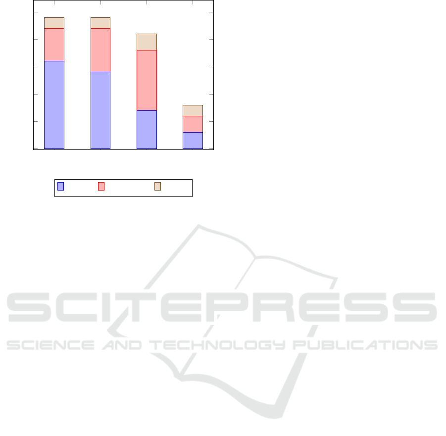
18-26 27-33 34-44 49-63
0
5
10
15
20
25
2 2
3
2
6
8
11
3
16
14
7
3
# of subjects
Normal Overweight Obese
Figure 1: Distribution of BMI groups over age groups.
5 CONCLUSION
This study provides some basis for the selection of
sampling rates and window sizes for human activity
recognition. The analysis indicates that 10s/50Hz is
statistically the best combination for data collected
with a single hip-worn accelerometer. Most of the ex-
periments carried out preferred larger windows and
high sampling rates though some low intensity ac-
tivities and demographics can perform better with
smaller windows. Our analysis further suggests that
window size can vary between 2-10 seconds and sam-
pling rate 25-100Hz for different situations without
a significant loss in performance. While our study
has shown that larger windows are preferable, smaller
windows can still provide significant results if power
consumption is an issue. Additionally, lower values
are preferable for studies involving the less dynamic
activities or subjects who are more liable to be less
active.
Future work in this field should be done to un-
derstand aspects of Human Activity Recognition bet-
ter. This study was performed under some assump-
tions that can be scrutinized. The placement of the
accelerometer could be shown to affect classifier per-
formance for different activities — a combination of
sensors can also be used. Other sensors, such as heart
rate monitors or video image processors, provide new
avenues. This study can also be replicated using dif-
ferent classifiers or learning methods with different
feature sets. Extensive analysis on the statistical value
of other machine learning and data mining methods
could also help the field as a whole.
REFERENCES
ActiGraph. Actisoft analysis software 3.2 user’s manual.
fort walton beach, fl: Mti health services.
Banos, O., Galvez, J.-M., Miguel Damas, H. P., and Ro-
jas, I. (2014). Window size impact in human activity
recognition. Sensors, pages 6474–6499.
Beiber, G., Voskamp, J., and Urban, B. (2009). Activity
recognition for everyday life on mobile phones. Inter-
national Conference on Universal Access in Human-
Computer Interaction, pages 289–296.
Demsar, J. (2006). Statistical comparisons of classifiers
over multiple data sets. Journal of Machine Learning
Research, 7:1–30.
Hall, M., Frank, E., Holmes, G., Pfahringer, B., Reutemann,
P., and Witten, I. H. (2009). The weka data min-
ing software: An update. SIGKDD Explor. Newsl.,
11(1):10–18.
Lara, O. D. and Labrador, M. A. (2013). A survey
on human activity recognition using wearable sen-
sors. IEEE Communication Surveys and Tutorials,
15:1192–1209.
Lau, S. and David, K. (2010). Movement recognition us-
ing the accelerometer in smartphones. IEEE Future
Network ands Mobile Summit 2010, pages 1–9.
Maurer, U., Smailagic, A., Siewiorek, D. P., and Deisher,
M. (2006). Activity recognition and monitoring using
multiple sensors on different body position. Interna-
tional Workshop on Wearable and Implantable Body
Sensor Networks.
Niazi, A., Yazdensepas, D., Gay, J., Maier, F., Rasheed, K.,
Ramaswamy, L., and Buman, M. (2016). A hierar-
chical meta-classifier for human activity recognition.
IEEE International Conference on Machine Learning
and Applications.
Preece, S. J., Goulermas, J. Y., Kenney, L. P. J., Howard,
D., Meijer, K., and Crompton, R. (2009). Activ-
ity identification using body-mounted sensorsa review
of classification techniques. Physiological Measure-
ment, 30(4):R1.
RStudio Team (2015). RStudio: Integrated Development
Environment for R. RStudio, Inc., Boston, MA.
Tapia, E., Intille, S., Haskell, W., Larson, K., Wright, J.,
King, A., and Friedman, R. (2007). Real-time recog-
nition of physical activities and their intensities us-
ing wireless accelerometers and a heart rate monitor.
IEEE 11th IEEE international symposium on wear-
able computers, pages 37–40.
Yazdansepas, D., Niazi, A. H., Gay, J. L., Maier, F. W., Ra-
maswamy, L., Rasheed, K., and Buman, M. P. (2016).
A multi-featured approach for wearable sensor-based
human activity recognition. IEEE International Con-
ference on Healthcare Informatics (ICHI), Chicago,
IL.
Statistical Analysis of Window Sizes and Sampling Rates in Human Activity Recognition
325
