Flow Parameters Derived from Impedance Pneumography after

Nonlinear Calibration based on Neural Networks

Marcel Mły

nczak

and Gerard Cybulski

1,2

Institute of Metrology and Biomedical Engineering, Faculty of Mechatronics, Warsaw University of Technology,

Boboli 8, 02-525, Warsaw, Poland

Department of Applied Physiology, Mossakowski Medical Research Centre, Polish Academy of Sciences,

Pawinskiego 5, 02-106 Warsaw, Poland

Keywords:

Ambulatory Monitoring, Impedance Pneumography, Calibration, Neural Networks.

Abstract:

Impedance pneumography (IP) is mainly used as a noninvasive method to measure respiratory rate, tidal

volume or minute ventilation. It could also register ﬂow-related signals, after differentiation, from spirometry-

based forced vital capacity maneuvers or ambulatory-based signals reﬂecting ﬂow values during natural activ-

ity. The aim of this paper is to assess the possibility of improving the accuracy of ﬂow parameters calculated

by IP, by using nonlinear neural network correction (as opposed to simple linear calibration), and to evaluate

the impact of various calibration procedures and neural network conﬁgurations. Ten students carried out ﬁxed

static breathing sequences, for both calibration and testing. A reference pneumotachometer and the Pneumoni-

tor 2 were used. The validation of calculating peak and mean ﬂow value during each inspiration and expiration

was considered. A mean accuracy of 80% was achieved for a separate neural network with two hidden layers

with 10 neurons in each layer, trained individually for each subject and body position, using the data from the

longest, ﬁxed calibration procedure. Simple linear modeling achieved only 72.5%.

1 INTRODUCTION

1.1 Problem and Related Works

Respiratory activity appears to be an important fac-

tor in physiological analyses, based on measurements

carried out both in the laboratory and under ambu-

latory conditions. Such studies need to extend be-

yond single spirometry evaluation, gathering the data

produced during natural functioning of the subjects

(Poupard et al., 2008; Koivumaki et al., 2012).

Impedance pneumography (IP) could be used to

measure ventilation non-invasively, even for long-

term monitoring, impacting the subject’s natural ac-

tivity during registration less than when using face

mask (Houtveen et al., 2006; Seppa et al., 2010;

Mły

nczak et al., 2015b).

Many studies have used impedance pneumog-

raphy to measure respiratory rate or tidal volume

(from which one could estimate minute ventilation)

(Houtveen et al., 2006; Seppa et al., 2010; Seppa

et al., 2011; Mły

nczak et al., 2015b; Mły

nczak et al.,

2015a; Gracia et al., 2015; Ansari et al., 2016). Those

three parameters are the main ones for respiratory

activity under unconstrained conditions, e.g., during

sleep (Roebuck et al., 2013; Seppa et al., 2016).

Impedance pneumography provides a volume-

related signal. However, it could also be used to mea-

sure ﬂow values after differentiation. This could be

used to assess spirometry-based parameters, recorded

during forced vital capacity (FVC) maneuver (Seppa

et al., 2013b), or to enhance the information derived

from ambulatory impedance measurement. In the sec-

ond condition, peak and mean ﬂow during each inspi-

ration and expiration could be calculated.

In a recent work, we assessed the accuracy and re-

producibility of linear calibration coefﬁcients on es-

timation of tidal volume from impedance pneumog-

raphy (Mły

nczak et al., 2015a). Our analysis found

greater error in the calculated ﬂow values than in

the calculated tidal volumes, compared to reference

pneumotachometry (PNT ). In most cases, the results

were underestimated, particularly for greater ﬂow val-

ues. This could imply that linear calibration of the

impedance signal cannot faithfully reﬂect changes

in ﬂow signal dynamics. Therefore, the assumption

made during volume calculations, that the best ﬁtting

could be provided by linear regression modeling, ap-

peared to be wrong.

MÅ

CyÅ

Dczak M. and Cybulski G.

Flow Parameters Derived from Impedance Pneumography after Nonlinear Calibration based on Neural Networks.

DOI: 10.5220/0006146800700077

In Proceedings of the 10th International Joint Conference on Biomedical Engineering Systems and Technologies (BIOSTEC 2017), pages 70-77

ISBN: 978-989-758-212-7

One of the possibilities to deal with this prob-

lem are hardware solutions, e.g., applying more so-

phisticated multifrequency application current signals

(multi-sinusoidal or binary one, with speciﬁc peaks of

frequencies) (Ojarand et al., 2013; Min and Paavle,

2013).

The other possibility may include an implemen-

tation of the more advanced signal processing of the

IP signal, including the way of handling the cardiac

component or the calibration strategy (the sequence

of differentiation and modeling in relation to the ref-

erence data).

Further, nonlinear corrections might be applied in

order to handle better signal dynamics. Artiﬁcial neu-

ral networks have been already used in other scientiﬁc

disciplines for such issue (Lai et al., 2015; Li et al.,

2015). They are also increasingly used in the analysis

of respiratory system activity in general (Jafari et al.,

2010; Lee et al., 2012; Baemani et al., 2008).

1.2 Objectives

The main objective of this paper is to assess the pos-

sibility of improving the accuracy of ﬂow parame-

ters calculated by impedance pneumography, by us-

ing nonlinear neural-network correction (as opposed

to the simple linear model), based on ﬂow-related sig-

nals.

The associated goals are to evaluate, what calibra-

tion procedure could provide the best data, leading

to the best accuracy in subsequent measurement anal-

ysis, and what neural network structure and order of

corrections is the most suitable for analysis of the ﬂow

parameters.

2 METHODS

2.1 Subjects & Devices

Basic information about the study participants is pro-

vided in Table 1. All were generally healthy male stu-

dents (without any respiratory disease reported) and

were informed about the aim of the measurements and

gave written consent.

Table 1: Information about the study participants.

Minimum Mean Maximum

Weight [kg] 65.0 77.4 100.0

Height [cm] 171.0 179.3 187.0

BMI 20.75 24.14 33.41

Age 19 23 27

We used our impedance pneumography prototype,

Pneumonitor 2, to measure IP signals. We used the

tetrapolar method, in which two electrodes apply a

current signal and the remaining two measure volt-

age, which is related to the electrical impedance. The

conﬁguration proposed by Seppa et al. was utilized

(Seppa et al., 2013a): receiving electrodes were posi-

tioned on the midaxillary line at about 5th-rib level,

and application electrodes on the same level on the

inner arms.

The Flow Measurement System (by Medikro Oy,

Kuopio, Finland) with a Spirometer Unit (M909), a

Fleisch-type Heatable Flow Transducer (5530), and a

Conical Mouthpiece (M9114), without any resistance,

were used as a reference PNT device. A 3L syringe

was used for daily system calibration to ensure accu-

rate ﬂow values.

The sampling frequency of the reference PNT sig-

nal was 200Hz, while that of the Pneumonitor 2 is

= 250Hz. All signals were transformed (via inter-

polation) to the latter frequency.

2.2 Protocol & Analysis

The calibration was performed for three body posi-

tions (supine, sitting and standing), due to the signif-

icant impact of body posture on the calibration coef-

ﬁcients (Mły

nczak et al., 2015b). Data for each po-

sition were gathered with three different calibration

protocols, differing by the duration of registration and

breathing regularity:

• free breathing registered for 30 seconds, hereafter

called ’Calibration Procedure 1’,

• free breathing recorded for 2 minutes, hereafter

called ’Calibration Procedure 2’, and

• ﬁxed breathing, alternately shallow and deep, 4

breaths of each, for each of three frequencies, 6,

10, and 15 breaths per minute (BPM), to evalu-

ate whether signals containing various breathing

dynamics (rates and depths) may improve the cal-

ibration of ﬂow-related signals, hereafter called

’Calibration Procedure 3’.

Data for testing were obtained with a fourth pro-

cedure, consisting of 6 normal breaths followed by 6

deep breaths (the difference in depth was subjective),

for three breathing rates (6, 10 and 15 BPM) and for

three body positions (the same as during each cali-

bration procedure). We automatically marked the ref-

erence breathing phases (inspiration, expiration, and

breathing pause) for each recording using simple am-

plitude thresholding of the ﬂow-related raw PNT sig-

nal. We also included in the algorithm heuristics to

remove artifacts, very short phases and errors.

Flow Parameters Derived from Impedance Pneumography after Nonlinear Calibration based on Neural Networks

Both calibration and test IP signals were pro-

cessed by subtracting the noise component produced

by least mean square adaptive ﬁltration from the raw

IP signal, then smoothing the difference with a 400

ms window. Then, ﬂow-related signals were obtained

by second-order differentiation of all IP signals. After

differentiation, a simple moving-average smoothing

method with a 500 ms window was applied, striking

a balance between (necessary) removal of the cardiac

component and (undesirable) deterioration of the sig-

nal dynamics.

The basic calibration could be performed by cal-

culating the single linear coefﬁcient between the

PNT reference and the processed, ﬂow-related, IP-

differentiated signal, without needing to take into ac-

count the intercept coefﬁcient of the linear model.

However, linear calibration for ﬂow signals provides

much worse accuracy than for volume signals. In-

stead, we implemented nonlinear improvement, based

on neural networks, using the MATLAB Neural Net-

work Fitting App (described more precisely in the

next section) (Mathworks, 2016).

In order to compare ﬂow parameters, absolute and

relative errors of maximum ﬂow during inspiration (as

a positive value), maximum ﬂow during expiration (as

a negative value), and mean ﬂow values during each

phase, were calculated. We also provided T-test anal-

ysis to evaluate, whether the differences were statis-

tically signiﬁcant, as well as box, compatibility, and

Bland-Altman plots.

Since some artifacts and very quick, unrepresen-

tative breathing phases remained after automatic seg-

mentation, we also provided the analysis after remov-

ing 5% outliers, from the inspiration and expiration

data, based on the reference PNT signal.

All analyses were performed using MATLAB.

2.3 Neural Network Correction

To ﬁt the neural network, a basic perceptron archi-

tecture (with single-element-vector input, speciﬁc

numbers of sigmoid hidden layers and neurons in

those layers, and a linear output layer) was applied,

taking randomly selected signal samples in each it-

eration. IP was treated as input, and PNT as refer-

ence/output. During learning procedure the classic

Levenberg-Marquardt back-propagation method

was used, we chose the default division of calibra-

tion data into training (70%), validation (15%), and

test sets (15%).

We evaluated 13 approaches, listed below. ”Indi-

vidual training” refers to the separate use of the data

for each participant, for every calibration procedure

and for every body position, as input for a neural net-

work. ”Global training” indicates that the signals for

all conditions were combined and single neural net-

work was calculated.

1. Only simple linear modeling based on ﬂow-

related signals.

2. Neural network with a single hidden layer with

10 neurons, trained individually.

3. Neural network with a single hidden layer with

20 neurons, trained individually.

4. Neural network with two hidden layers of 5 neu-

rons each, trained individually.

5. Neural network with two hidden layers of 10

neurons each, trained individually.

6. Simple linear modeling and then neural network

with a single hidden layer with 10 neurons,

trained individually.

7. Simple linear modeling and then neural network

with a single hidden layer with 20 neurons,

trained individually.

8. Simple linear modeling and then neural network

with two hidden layers of 5 neurons each,

trained individually.

9. Simple linear modeling and then neural network

with two hidden layers of 10 neurons each,

trained individually.

10. Simple linear modeling and then neural network

with a single hidden layer with 10 neurons,

trained globally.

11. Simple linear modeling and then neural network

with a single hidden layer with 20 neurons,

trained globally.

12. Simple linear modeling and then neural network

with two hidden layers of 5 neurons each,

trained globally.

13. Simple linear modeling and then neural network

with two hidden layers of 10 neurons each,

trained globally.

Those calibration approaches were performed for

signals obtained during each breathing protocol and

for all three body positions. In each case, we used

the Levenberg-Marquardt back-propagation learning

method. The neural networks’ architectures were set

arbitrarily, in order to evaluate their possible impact

on accuracy and learning time.

Due to the fact that the result of the neural network

training could be ”discontinuous”, we performed full

accuracy analysis for the best calibration procedure

with the addition of moving-average smoothing at the

end of the calibration calculations (with an arbitrary

window of 200 ms).

BIOSIGNALS 2017 - 10th International Conference on Bio-inspired Systems and Signal Processing

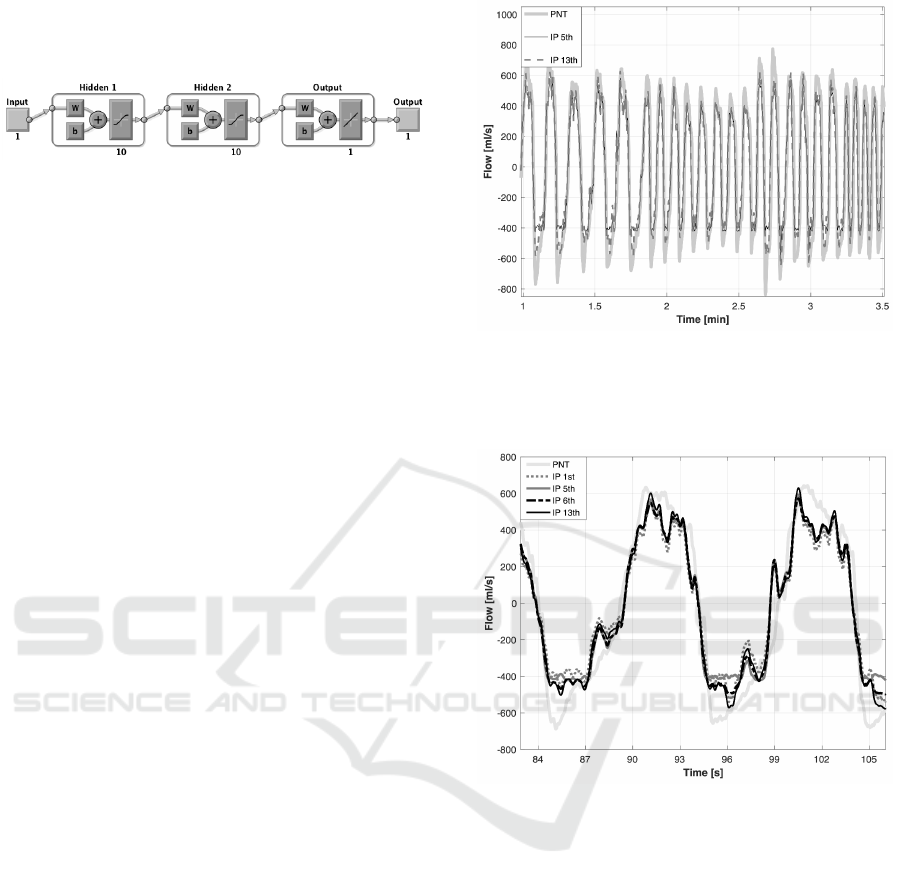
As an example, the neural network architecture

from the ﬁfth approach is presented in Fig. 1.

Figure 1: Neural network architecture from the ﬁfth ap-

proach (enumerated earlier); abbreviations: W - weight ma-

trix, b - bias vector (Mathworks, 2016).

3 RESULTS

A sample relationship between the reference PNT

signal and the ﬂow-related IP signal, calculated by

the 5th, and 13th calibration approaches, for the sec-

ond participant in the sitting position, is presented in

Fig. 2. An excerpt of those signals (adding the ones

for the 1st and 6th calibration approaches), represent-

ing two consecutive breaths, is shown in Fig. 3.

Tables 2, 3, and 4 each present the absolute er-

rors, relative errors, and p-values of the maximum and

mean ﬂow parameters for Calibration Procedures 1,

2, and 3, respectively (out of the 13 approaches, only

the 9 with the best outcomes for each procedure are

shown). For the best calibration procedure, we also

performed the analysis with smoothed calibration re-

sults (with a 200 ms window, hereafter called post-

hoc smoothing). The results appear in Table 5.

We did not observe any one participant sig-

niﬁcantly contributing to the decrease in accuracy.

The ﬂow parameters with the smallest overall error

were calculated for Calibration Procedure 3, with

the 6th calibration approach without any other post-

processing, and with the 5th with post-hoc smooth-

ing. It is worth noting that adding the smoothing to

the calibration result slightly increased the accuracy,

particularly for those calibration approaches in which

individually trained neural networks were used.

Generally, combining calculations for peak and

mean ﬂow values, Calibration Procedure 3 and the 5th

calibration approach seemed best, with 80% mean ac-

curacy, compared to 72.5% for simple linear calibra-

tion.

We observed no statistically signiﬁcant corre-

spondence between ﬂow parameters using the ﬁrst

calibration approach (only simple linear modeling).

More complicated calibration procedures yielded

lower numbers of neural-network-based approaches

in which there was statistically signiﬁcant correspon-

dence between ﬂow parameters. For the best combi-

nation, the differences in peak ﬂow calculations were

statistically signiﬁcant.

Figure 2: Sample comparison of the 5th, and 13th calibra-

tion approach results, calculated from the IP signal, in rela-

tion to the reference PNT signal, for the ﬁrst participant in

a sitting position.

Figure 3: Excerpt of the sample comparison of the 1st, 5th,

6th, and 13th calibration approach results, calculated from

the IP signal, relative to the reference PNT signal, for the

ﬁrst participant, sitting.

Individual neural-network learning was over 14

times faster than global one, comparing 36 seconds to

4 minutes and 12 seconds, on average, respectively.

The processing times were measured with the com-

puter processor Intel i5 (1200 MHz), with automati-

cally activated accelerations (up to 2700 MHz).

The box, compatibility, and Bland-Altman plots

for the calculated maximum ﬂows for Calibration

Procedure 3 and the 6th calibration approach are pre-

sented in Fig. 4, 5, and 6, respectively. The same

analysis was provided for the 5th calibration approach

after applying post-hoc smoothing. The correspond-

ing box, compatibility, and Bland-Altman plots are

shown in Fig. 7, 8, and 9, respectively.

Flow Parameters Derived from Impedance Pneumography after Nonlinear Calibration based on Neural Networks

Table 2: Comparison of the maximum and mean ﬂow values for the 9 most accurate approaches (considering average error

from maximum and mean ﬂow calculations) for Calibration Procedure 1; A - absolute error in milliliters per second; R -

relative error in percents; p - approximate p-value of paired T test, accurate to the hundredths.

Calibration Approach

1 4 5 6 9 10 11 12 13

Max

Flow

A 200.7 246.3 220.9 216.7 233.1 178.9 174.3 175.1 173.6

R 34.6 35.9 31.3 30.9 33.5 25.5 24.8 24.9 24.8

p 0.09 <0.01 <0.01 <0.01 <0.01 <0.01 <0.01 <0.01 <0.01

Mean

Flow

A 187.6 182.1 169.8 173.5 189.6 145.6 145.2 145.8 145.2

R 43.7 38.2 34.0 34.1 37.9 30.7 30.3 30.4 30.3

p 0.58 <0.01 <0.01 <0.01 <0.01 <0.01 <0.01 <0.01 <0.01

Table 3: Comparison of the maximum and mean ﬂow values for the 9 most accurate approaches (considering average error

from maximum and mean ﬂow calculations) for Calibration Procedure 2; A - absolute error in milliliters per second; R -

relative error in percents; p - approximate p-value of paired T test, accurate to the hundredths.

Calibration Approach

1 2 5 6 9 10 11 12 13

Max

Flow

A 142.6 182.4 175.6 197.2 200.1 128.1 136.9 131.5 131.4

R 26.6 25.4 24.7 28.5 29.3 18.9 19.7 19.3 19.3

p 0.21 0.85 0.67 0.11 0.18 0.01 <0.01 <0.01 0.87

Mean

Flow

A 130.8 151.3 147.5 167.7 155.2 118.5 122.3 119.7 119.8

R 31.6 31.1 29.9 33.3 32.3 26.0 26.7 26.3 26.3

p 0.92 0.36 0.18 0.01 0.33 0.41 0.07 0.20 0.63

Table 4: Comparison of the maximum and mean ﬂow values for the 9 most accurate approaches (considering average error

from maximum and mean ﬂow calculations) for Calibration Procedure 3; A - absolute error in milliliters per second; R -

relative error in percents; p - approximate p-value of paired T test, accurate to the hundredths.

Calibration Approach

1 2 4 5 6 7 8 11 13

Max

Flow

A 144.3 126.8 132.3 118.4 118.5 120.7 118.9 133.0 134.3

R 28.6 21.1 22.6 20.9 20.8 22.9 20.0 23.9 24.3

p 0.37 0.04 0.04 0.05 <0.01 0.01 0.03 0.10 0.26

Mean

Flow

A 102.8 89.2 100.3 90.5 87.7 88.6 96.4 84.3 85.1

R 25.8 22.2 24.2 21.5 21.4 21.6 22.9 20.9 21.3

p 0.68 0.89 0.93 0.81 0.51 0.95 0.28 0.10 0.18

Table 5: Comparison of the maximum and mean ﬂow values for the 9 most accurate approaches (considering average error

from maximum and mean ﬂow calculations) for Calibration Procedure 3 after post-hoc smoothing of the calibration results

with a 200 ms window; A - absolute error in milliliters per second; R - relative error in percents; p - approximate p-value of

paired T test, accurate to the hundredths.

Calibration Approach

1 2 5 6 7 8 10 11 13

Max

Flow

A 144.3 119.0 109.1 109.7 110.0 113.6 130.5 123.7 125.3

R 28.6 19.5 18.4 19.0 19.3 18.7 22.8 21.6 22.3

p 0.37 0.04 <0.01 <0.01 <0.01 0.04 <0.01 0.18 0.36

Mean

Flow

A 102.8 90.1 91.4 88.6 89.5 97.4 87.9 85.0 85.9

R 25.8 23.4 21.6 21.7 22.0 23.2 22.4 21.0 21.4

p 0.68 0.88 0.80 0.50 0.93 0.28 0.01 0.10 0.18

BIOSIGNALS 2017 - 10th International Conference on Bio-inspired Systems and Signal Processing

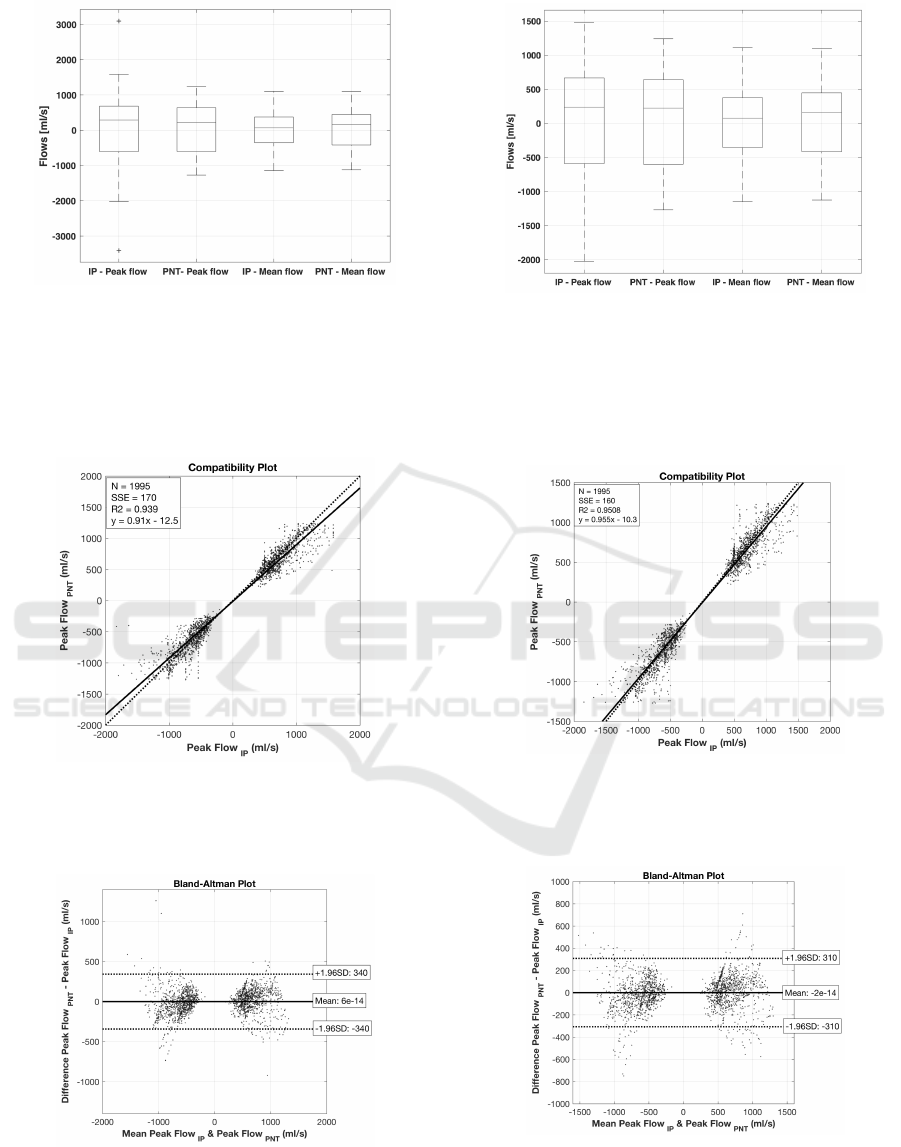
Figure 4: Box-plot comparing the maximum (peak) and

mean IP and PNT ﬂow values and the differences between

them, calculated for both inspirations and expirations, for

all participants and body positions, for Calibration Proce-

dure 3 and the 6th calibration approach; positive values

correspond to inspiration ﬂows, negative ones - to expira-

tion.

Figure 5: Compatibility plot for maximum ﬂows, calculated

for both inspirations and expirations, for all participants and

body positions, for Calibration Procedure 3 and the 6th cal-

ibration approach.

Figure 6: Bland-Altman plot for maximum ﬂows, calcu-

lated for both inspirations and expirations, for all partici-

pants and body positions, for Calibration Procedure 3 and

the 6th calibration approach.

Figure 7: Box-plot comparing the maximum (peak) and

mean IP and PNT ﬂow values and the differences between

them, calculated for both inspirations and expirations, for

all participants and body positions, for Calibration Proce-

dure 3 and the 5th calibration approach after post-hoc

smoothing; positive values correspond to inspiration ﬂows,

negative ones - to expiration.

Figure 8: Compatibility plot for maximum ﬂows, calculated

for both inspirations and expirations, for all participants and

body positions, for Calibration Procedure 3 and the 5th cal-

ibration approach after post-hoc smoothing.

Figure 9: Bland-Altman plot for maximum ﬂows, calcu-

lated for both inspirations and expirations, for all partici-

pants and body positions, for Calibration Procedure 3 and

the 5th calibration approach, after post-hoc smoothing.

Flow Parameters Derived from Impedance Pneumography after Nonlinear Calibration based on Neural Networks

4 DISCUSSION

In general, this paper touches the issue of improving

the accuracy of determining the respiratory ﬂow pa-

rameters. As the more advanced method, the elec-

trical impedance tomography seems to provide bet-

ter set of data to estimate ventilation and perfusion as

by using ”single” signal in impedance pneumography

(Leonhardt and Lachmann, 2012).

Nevertheless, in this paper we evaluated the im-

provement of peak and mean ﬂow estimation accu-

racy, using differentiated IP signal (convenient from

the point of view of long-term measurement), result-

ing from adding neural-network ﬁtting correction or

separate modeling. The idea of using the nonlinear

correction approach stemmed from the observation

that the largest divergence between IP and reference

signals seemed to be near the peak value.

The veriﬁcation was performed with different cali-

bration procedures (in order to check which one could

provide the best input data leading to the best results

during test measurements) and calibration approaches

(deﬁning the order of applying linear and neural-

network models), with post-hoc smoothing provided

for the best calibration procedure (to check the pos-

sible impact of appearance of the cardiac component

on the calculation).

We used neural networks individually (for speciﬁc

subject and body position data) or globally (gathering

all data), with or without previously applying linear

calibration coefﬁcients. The best accuracies were ob-

tained for Calibration Procedure 3, in which breath-

ing rates were ﬁxed and depths of breathing forced.

Among them, individually trained neural-network ap-

proaches seemed the best in each assessed aspect. The

necessity of linear modeling before neural network

ﬁtting remains important and in need of evaluation.

There is also the question of whether there is an opti-

mal network conﬁguration (number of hidden layers

and neurons per layer), or whether it is dependent on

the speciﬁc subject and measurements being evalu-

ated.

It is worth remembering that the neural-network

approach is based on random selection of the input

and target data in the learning process. Without set-

ting the seed beforehand, we are unable to obtain the

same ﬁt in subsequent repetitions of the training pro-

cess. Besides, the ﬁtting could be discontinuous (due

to the speciﬁc data, particularly when there is an ar-

tifact in the signals). The subtle post-hoc smoothing

was added to deal with that issue.

The individual approach to neural-network ﬁtting

reduces learning time. This could be useful with

regards to ambulatory monitoring and the prospect

of assessing different network conﬁgurations to see

which may be best suited to an individual.

The following limitations of this study require

mention:

• participants were only 10 males,

• measurements were carried out only under static

conditions,

• in ambulatory situations, recordings are longer

and more diversiﬁed, which may affect overall ac-

curacy,

• there was no distinction of breathing depths,

breathing rates, or body positions in the ﬂow ac-

curacy assessment; the results were gathered into

the one set, and

• the neural network approach is compared to the

use of simple linear modeling calibration coefﬁ-

cient; there is no comparative analysis with an-

other nonlinear methods.

Future plans include:

• assessing the accuracy for models established sep-

arately for inspirations and expirations, and for

different depth of breathing,

• validating the accuracy in the case of a different

order of differentiation and calibration (e.g., linear

or nonlinear calibration for volume-related data

with differentiation as a ﬁnal step, performed in

order to analyze ﬂow values),

• comparing the results from presented neural-

network-based approach with the ones derived

from different nonlinear correction algorithm,

• checking the possibility to improve the accuracy

by removing the cardiac component adaptively in

the way, that the dynamics of the signal changes

(particularly for higher ﬂows) is preserved in the

most optimal way, and

• evaluating more advanced methods of neural net-

work learning (Monteiro et al., 2016).

5 CONCLUSIONS

The following conclusions may be drawn:

• Non-linear neural-network-based correction of

the linear calibration model or a separate neural

network ﬁtting model can improve the mean accu-

racy of peak and mean ﬂow parameters calculated

from impedance pneumography signals.

• The longest considered calibration procedure,

consisting of ﬁxed breathing with different rates

BIOSIGNALS 2017 - 10th International Conference on Bio-inspired Systems and Signal Processing

and depths, allows better coverage of possible

ﬂow changes in test signals.

• Neural networks trained individually for every

body position of a particular subject seem to pro-

vide better results than ones trained with a global

set.

• We obtained 80% accuracy with the best combi-

nation (separate model based on a neural network

with two hidden layers of 10 neurons each, trained

individually on the data from 3rd calibration pro-

cedure), versus 72.5% for simple linear modeling.

ACKNOWLEDGMENTS

This study was supported by the research programs of

institutions the authors are afﬁliated with.

REFERENCES

Ansari, S., Ward, K., and Najarian, K. (2016). Motion Ar-

tifact Suppression in Impedance Pneumography Sig-

nal for Portable Monitoring of Respiration: an Adap-

tive Approach. IEEE J. Biomed. Heal. Informatics,

11(4):1–1.

Baemani, M. J., Monadjemi, A., and Moallem, P. (2008).

Detection of respiratory abnormalities using artiﬁ-

cial neural networks. Journal of Computer Science,

4(8):663–667.

Gracia, J., Seppa, V. P., and Viik, J. (2015). Regional

impedance pneumography heterogeneity during air-

way opening pressure chirp oscillations. Int. J. Bio-

electromagn., 17(1):42–51.

Houtveen, J. H., Groot, P. F. C., and De Geus, E. J. C.

(2006). Validation of the thoracic impedance derived

respiratory signal using multilevel analysis. Int. J.

Psychophysiol., 59(2):97–106.

Jafari, S., Arabalibeik, H., and Agin, K. (2010). Classiﬁca-

tion of normal and abnormal respiration patterns us-

ing ﬂow volume curve and neural network. In Health

Informatics and Bioinformatics (HIBIT), 2010 5th In-

ternational Symposium On, pages 110–113. IEEE.

Koivumaki, T., Vauhkonen, M., Kuikka, J. T., and Haku-

linen, M. a. (2012). Bioimpedance-based measure-

ment method for simultaneous acquisition of respi-

ratory and cardiac gating signals. Physiol. Meas.,

33(8):1323–1334.

Lai, C.-L., Lee, J.-S., and Chen, J.-C. (2015). A curve ﬁt-

ting approach using ann for converting ct number to

linear attenuation coefﬁcient for ct-based pet attenu-

ation correction. IEEE Transactions on Nuclear Sci-

ence, 62(1):164–170.

Lee, S. J., Motai, Y., Weiss, E., and Sun, S. S. (2012). Ir-

regular breathing classiﬁcation from multiple patient

datasets using neural networks. IEEE Transactions on

Information Technology in Biomedicine, 16(6):1253–

1264.

Leonhardt, S. and Lachmann, B. (2012). Electrical

impedance tomography: The holy grail of ventila-

tion and perfusion monitoring? Intensive Care Med.,

38:1917–1929.

Li, Y., Pan Fua, Z. L., Lia, X., and Lina, Z. (2015). Biax-

ial angle sensor calibration method based on artiﬁcial

neural network. Chemical Engineering, 46:361–366.

Mathworks (2016). Fit Data with a Neural Net-

work. https://www.mathworks.com/help/nnet/gs/ﬁt-

data-with-a-neural-network.html. [Online; accessed

07-October-2016].

Min, M. and Paavle, T. (2013). Improved extraction of in-

formation in bioimpedance measurements. In J. Phys.

Conf. Ser., volume 434, pages 0120291–4.

Mły

nczak, M., Niewiadomski, W.,

Zyli

nski, M., and Cybul-

ski, G. (2015a). Assessment of calibration methods

on impedance pneumography accuracy. Biomed. Eng.

/ Biomed. Tech.

Mły

nczak, M., Niewiadomski, W.,

Zyli

nski, M., and Cybul-

ski, G. (2015b). Veriﬁcation of the Respiratory Param-

eters Derived from Impedance Pnumography during

Normal and Deep Breathing in Three Body Postures.

In IFMBE Proc., volume 45, pages 162–165.

Monteiro, R. L. S., Carneiro, T. K. G., Fontoura, J. R. A.,

Da Silva, V. L., Moret, M. A., and De Barros Pereira,

H. B. (2016). A model for improving the learning

curves of artiﬁcial neural networks. PLoS One, 11(2).

Ojarand, J., Annus, P., and Min, M. (2013). Optimisation of

multisine waveform for bio-impedance spectroscopy.

In J. Phys. Conf. Ser., volume 434, pages 0120301–4.

Poupard, L., Mathieu, M., Sart

ene, R., and Goldman, M.

(2008). Use of thoracic impedance sensors to screen

for sleep-disordered breathing in patients with cardio-

vascular disease. Physiol. Meas., 29(2):255–267.

Roebuck, A., Monasterio, V., Gederi, E., Osipov, M., Behar,

J., Malhotra, A., Penzel, T., and Clifford, G. (2013). A

review of signals used in sleep analysis. Physiological

measurement, 35(1):R1.

Seppa, V. P., Hyttinen, J., Uitto, M., Chrapek, W., and

Viik, J. (2013a). Novel electrode conﬁguration for

highly linear impedance pneumography. Biomed. Eng.

/ Biomed. Tech., 58(1):35–38.

Seppa, V.-P., Hyttinen, J., and Viik, J. (2011). A method

for suppressing cardiogenic oscillations in impedance

pneumography. Physiol. Meas., 32(3):337–345.

Seppa, V.-P., Pelkonen, A. S., Kotaniemi-Syrjanen, A.,

Makela, M. J., Viik, J., and Malmberg, L. P. (2013b).

Tidal breathing ﬂow measurement in awake young

children by using impedance pneumography. J. Appl.

Physiol., 115(11):1725–31.

Seppa, V.-P., Pelkonen, A. S., Kotaniemi-Syrjanen, A.,

Viik, J., Makela, M. J., and Malmberg, L. P. (2016).

Tidal ﬂow variability measured by impedance pneu-

mography relates to childhood asthma risk. Eur.

Respir. J., pages 1–10.

Seppa, V.-P., Viik, J., and Hyttinen, J. (2010). Assessment

of pulmonary ﬂow using impedance pneumography.

IEEE Trans. Biomed. Eng., 57(9):2277–2285.

Flow Parameters Derived from Impedance Pneumography after Nonlinear Calibration based on Neural Networks