Performance Analysis of Spatial Laser Speckle Contrast

Implementations

Pedro G. Vaz

1,2

, Anne Humeau-Heurtier

, Edite Figueiras

, Carlos Correia

and Jo

ao Cardoso

LIBPhys-UC, Department of Physics, University of Coimbra, R. Larga, 3004-516 Coimbra, Portugal

University of Angers, LARIS - Laboratoire Angevin de Recherche en Ing

enierie des Syst

emes,

62 avenue Notre-Dame du Lac, 49000 Angers, France

International Iberian Nanotechnology Laboratory, Ultrafast Bio and Nanophotonics Group, Braga, Portugal

Keywords:

Laser Speckle Imaging, Spatial Contrast, Algorithm Implementation, MATLAB, Convolution.

Abstract:

This work presents an analysis of the performances for four different implementations used to compute laser

speckle contrast on images. Laser speckle contrast is a widely used imaging technique for biomedical appli-

cations. These implementations were tested using synthetic laser speckle patterns with different resolutions,

speckle sizes, and contrasts. From the applied methods, three implementations are already known in the

literature. A new alternative is proposed herein, which relies on two-dimensional convolutions, in order to

improve the image processing time without compromising the contrast assessment. The proposed implemen-

tation achieves a processing time two orders of magnitude lower than the analytical evaluation. The goal of

this technical manuscript is to help the developers and researchers in computing laser speckle contrast images.

1 INTRODUCTION

Laser speckle is an interference phenomenon that oc-

curs when coherent light is used to illuminate a sam-

ple. This interference is characterized by the visu-

alization of bright and dark spots which are called

speckles (Briers et al., 2013). Figure 1 shows an

example of a laser speckle image. The bright and

dark spots can vary in size and shape, depending on

the used sample, coherent light source and imaging

system. This image has been sensitized using the

algorithm detailed in (Kirkpatrick et al., 2007) and

presents a situation with a speckle size of 8 pixels per

speckle.

The laser speckle effect is widely used in biomed-

ical applications as a tool to assess the blood perfu-

sion (Briers et al., 2013). Its utilization fall from the

idea that, when a moving scatterer is presented in the

analysed sample, the speckle pattern will change over

time. The temporal speckle variations encode infor-

mation that can be related with the velocity of the dy-

namic scatterers. The analysis of laser speckle pat-

terns over time is called dynamic laser speckle (Vaz

et al., 2016a).

Normally, a two-dimensional imaging system,

with ﬁnite exposure time, is used to record these

speckle patterns along time resulting in a video struc-

ture. This information can be analysed by different

ways. On one hand, these changes can be identi-

ﬁed by comparing two consecutive speckle patterns.

On the other hand, the speckle pattern can be anal-

ysed by computing its contrast using a method often

called Laser Speckle Contrast Imaging (LSCI) (Drai-

jer et al., 2009). The pattern contrast is related with

the movement of the scatterers present in the sam-

ple. Faster scatterers mean faster image decorrelation

leading to lower contrast (Briers and Webster, 1996).

When this technique is applied to biomedical sam-

ples, like cerebral tissue, the moving scatterers are

mainly the red blood cells. As a consequence of the

speckle behaviour, the contrast of the laser speckle

pattern can be related with the tissue blood perfusion

(Vaz et al., 2016b). The speckle contrast is usually

computed in smaller regions of interest (ROI’s) in or-

der to achieve a two-dimensional contrast map. Laser

speckle is able to produce two-dimensional perfusion

maps in real-time (Humeau-Heurtier et al., 2013) and

with frame rates above 100 frames per second (Tom

et al., 2008) at a fair cost.

Speckle contrast can be computed using three dif-

ferent algorithms (Vaz et al., 2016b): the ﬁrst one uses

a spatial-based contrast computation, the second one

uses a temporal-based computation and, ﬁnally, the

last one combines the two previous families.

148

Vaz P., Humeau-Heurtier A., Figueiras E., Correia C. and Cardoso J.

Performance Analysis of Spatial Laser Speckle Contrast Implementations.

DOI: 10.5220/0006141101480153

In Proceedings of the 10th International Joint Conference on Biomedical Engineering Systems and Technologies (BIOSTEC 2017), pages 148-153

ISBN: 978-989-758-214-1

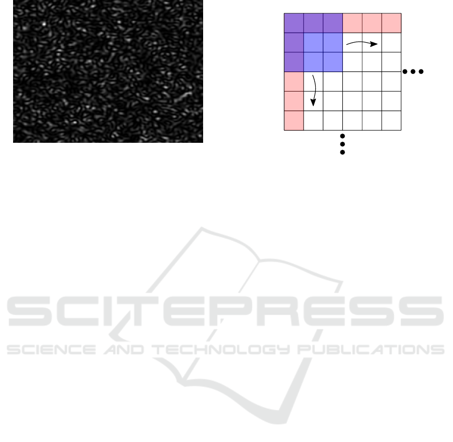
Figure 1: Synthetic laser speckle image with resolution of

320 × 240 pixels and a spot size of 8 pixels per speckle.

LSCI is used as a clinical and research tool in

many different types of tissues and diseases. Most

of the blood ﬂow analyses performed with LSCI are

related with highly vascularized tissues, like cerebral

tissues (Kazmi et al., 2015), retinal tissues (Cheng

and Duong, 2007) and hepatic tissues (Sturesson

et al., 2013). However, more recently, the assess-

ment of low vascularized tissues, like the skin, be-

came also a major ﬁeld of the application of LSCI

(Humeau-Heurtier et al., 2013; Roustit et al., 2010).

In this type of samples, studies on disorders like sys-

temic sclerosis (Ruaro et al., 2013), port wine stains

(Huang et al., 2009) and wound healing (Rege et al.,

2012) have been performed using laser speckle imag-

ing methods.

In this work, we propose to test the performance

of a set of spatial-based contrast implementations. We

will focus on this family because it is the most often

used. When computing the contrast spatially a small

two-dimensional ROI is used on the raw images. This

ROI is translated along the laser speckle image (LS

image) in the horizontal and vertical directions, gen-

erally without overlapping. Figure 2 presents an illus-

tration of the spatial contrast algorithm.

The ROI is usually deﬁned as a square of 3×3

(Pericam PSI documentation (Perimed AB, 2015)),

5×5 or 7×7 pixels (Draijer et al., 2009). The con-

trast is computed using the fundamental equation K =

σ(I)/hIi where σ(I) represents the standard deviation

of the intensity and hIi the mean intensity within the

ROI (Briers and Webster, 1996).

When online applications are necessary, or large

images are analysed, computational speed is a key

factor. The goal of this work is to explore different

spatial contrast implementations in order to determine

which one can achieve the best performance. This

paper will aid researchers to select the suitable im-

plementation depending on their requirements and to

i-1

i+1

j-1

j+1

Figure 2: Schematic of spatial contrast algorithm. The blue

square symbolizes a 3×3 ROI. Its contrast value is asso-

ciated with the raw image pixel (i,j). This ROI is trans-

lated along the lines and columns of the speckle image.

The red lines correspond to boundary regions where con-

trast determination requires padding. Adapted from (Vaz

et al., 2016b) with authors permission.

enlarge their implementations possibilities.

MATLAB



has been selected as a tool to test the

different algorithm implementations. MATLAB



a mathematical computing software, widely used in

research for signal processing due to its rapid learn-

ing curve and large range of pre-implemented func-

tions. The selected implementations, used to compute

speckle contrast, correspond to methods presented in

the literature (Steimers et al., 2016). Some implemen-

tations correspond to works previously performed

(Duncan and Kirkpatrick, 2008; Steimers et al., 2016)

and one corresponds to a novel implementation (sub-

section 2.4).

The performance results should be taken as spe-

ciﬁc for these experimental conditions, however these

conclusions might be applied for other software and

hardware platforms. The different implementations

were tested using synthetic LS images produced us-

ing the method presented by Kirkpatrick et al. (Kirk-

patrick et al., 2007).

2 METHODS

Four different implementations were developed in

MATLAB R2016a-64 bits. The ﬁrst one corresponds

to an analytical evaluation of the contrast equation

and was used as a reference. The second one is based

on image ﬁltering (Duncan and Kirkpatrick, 2008).

The third one relies on a moving sums (Steimers et al.,

2016). The fourth one uses convolution. The process-

ing time of each implementation was analysed using

different LS images and different ROI sizes.

Performance Analysis of Spatial Laser Speckle Contrast Implementations

149

LS images were synthesized with resolutions

of 320×240, 640×480, and 1024×768 pixels and

speckle sizes of 4, 8, 16, and 32 pixels. The applied

ROI’s have been deﬁned as squares of 3×3, 5×5 or

7×7 pixels. For each resolution, 200 different random

generated images were used, 50 for each speckle size,

and the computation time was determined as mean ±

standard deviation. The FLoating-point Operations

Per Second (FLOPS) were not computed because this

command is no longer available in MATLAB after

version R13SP2.

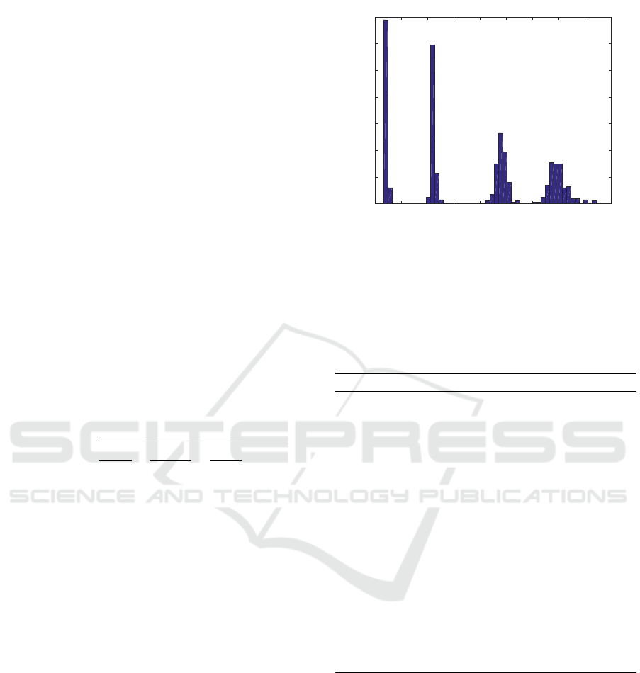
These images were ﬁltered with an average ﬁlter

in order to uniform their contrast. Figure 3 shows

the global contrast distribution of the 600 images that

were analysed in this work. This contrast exceeds the

maximum theoretical laser speckle contrast due to the

nature of the synthesis algorithm (Duncan and Kirk-

patrick, 2008). None attempt has been made to cor-

rect this contrast overshoot in order to allow for other

authors to follow the same protocol.

The ﬁrst implementation (section 2.1) is based on

the application of the contrast formula K = σ(I)/hIi

to compute the output data. The other three (sec-

tions 2.2, 2.3, and 2.4) are based on a modiﬁed for-

mula which replaces the standard deviation by inten-

sity sums (Steimers et al., 2016):

K =

N − 1

∑



∑



−

N − 1

, (1)

where N is the number of summed points. While the

standard equation requires to compute both the mean

and standard deviation of the ROI, equation (1) only

requires to sum the pixels of the LS image and of its

square. With this new equation, the spatial-contrast

algorithm can be implemented in an optimized way.

The use of the modiﬁed contrast equation (Eq.

(1)) presents a practical issue that should be discussed

before its application. The square root operation can

lead to imaginary values when its radicand is lower

than 0. Rearranging the square root radicand we ob-

tain that this equation is only valid if

∑

≥

1/N. This condition must be checked before the ap-

plication of this equation.

2.1 Analytical Computation

The analytical computation corresponds to the direct

application of the contrast equation in each ROI. The

mean intensity and standard deviation in each ROI

were computed using the functions std2 and mean2.

The ROI was applied to the entire LS image with-

out overlapping, by using two For cycles (one for the

rows and the other for the columns). The application

0.2 0.3 0.4 0.5 0.6 0.7 0.8 0.9 1 1.1

Contrast

100

120

140

Number of Images

Figure 3: Distribution of the average contrast values of all

the tested images. Total number of images: 600 frames.

of this process results in a reduction of the original

image resolution depending on the ROI size. This im-

plementation was not optimized and has been used as

the reference method.

Algorithm 1: Analytical computation.

Input: LS raw image (LSimage) and element size

(ROIsize)

Output: Contrast image (cImage)

for ii ← 1 to # of LSimage lines with ROIsize steps

for jj ← 1 to # of LSimage columns with ROI-

size steps do

ROI ← cut subimage with input size and the

pixel center in the position (ii,jj)

mean ← mean2(ROI)

std ← std2(ROI)

contrast ← std/mean

cImage ← contrast is stored in the correct po-

sition of the cImage

end for

return cImage

2.2 Filtering Implementation

The ﬁltering implementation consists in the applica-

tion of two images ﬁlters to the LS image. A regu-

lar ﬁlter, imfilter, with a kernel equal to the ROI

was applied in order to compute the LS image sum

and LS image squared sum. These data were then

used to evaluate Eq. (1). The original implementation

has been performed using MATLAB



(Duncan and

Kirkpatrick, 2008). This implementation is detailed

in pseudo-code in algorithm 2.

BIOINFORMATICS 2017 - 8th International Conference on Bioinformatics Models, Methods and Algorithms

150

Algorithm 2: FILTERING.

Input: LS raw image (LSimage) and element size

(ROIsize)

Output: Contrast image (cImage)

Kernel ← all-ones matrix with the ROIsize

Sum ← imﬁlter(LSimage, Kernel)

Sum2 ← imﬁlter(LSimage

, Kernel)

cImage ← application of the sums equation for each

point (Eq. 1)

return cImage

2.3 Moving Sum Implementation

The moving sum implementation has been described

in (Steimers et al., 2016) and (Tom et al., 2008). The

original algorithms were implemented in CUDA and

C programming languages. Hence, an adaptation of

this algorithm was implemented in MATLAB



. This

implementation aims at computing the sums of Eq.

(1) by performing a moving sum within the lines of

the LS image and a moving sum in the columns of

the resultant matrix. The moving sum was achieved

by using the movsum function. This implementation

is described in pseudo-code in algorithm 3.

Algorithm 3: MOVING SUM.

Input: LS raw image (LSimage) and element size

(ROIsize)

Output: Contrast image (cImage)

SumLines ← movsum(LSimage, ROIsize) for each

line

SumLines2 ← movsum(LSimage.∗ LSimage) for each

line

Sum ← movsum(movSumLines, ROIsize) for each

column

Sum2 ← movsum(movSumLines2, ROIsize) for each

column

cImage ← application of the sums equation for each

point (Eq. 1)

return cImage

2.4 Convolution Implementation

The two-dimensional convolution has been computed

using conv2 MATLAB



function. With this method,

equation (1) can easily be computed. Both sums were

computed by performing a convolution of the LS raw

image with a all-ones matrix with size equal to the

ROI. conv2 uses the algorithm presented in equa-

tion (2). This MATLAB



function has also been

tested against an equivalent method (convolution by

fast Fourier transform) and presented the best results.

This implementation is described in pseudo-code in

algorithm 4.

c(n1,n2) =

∞

∑

k1=−∞

∞

∑

k2=−∞

(k1, k2)I

(n1−k1,n2−k2) (2)

Algorithm 4: CONVOLUTION.

Input: LS raw image (LSimage) and element size

(ROIsize)

Output: Contrast image (cImage)

Kernel ← all-ones matrix with size equals to ROIsize

Sum ← conv2(LSimage, Kernel)

Sum2 ← conv2(LSimage. ∗ LSimage, Kernel)

cImage ← application of the sums equation for each

point (Eq. 1)

return cImage

3 PERFORMANCE RESULTS

The results were analysed in terms of image reso-

lution and ROI size. All the tests were performed

in a computer Toshiba Tecra S11-11G - i7 M620 @

2.67GHz with 4GB RAM with Windows 10 Pro as

operating system. The results (ﬁgure 4) show that the

convolution implementation achieves the best perfor-

mance in all the cases, followed by the ﬁltering algo-

rithm.

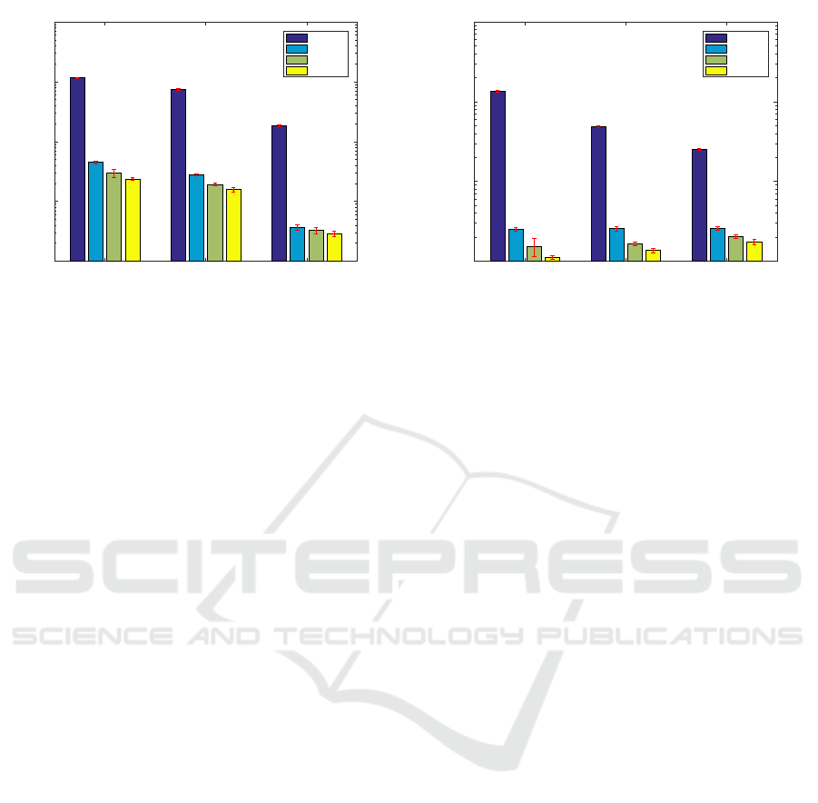
The results are summarized in ﬁgure 4. This ﬁg-

ure shows the computation time needed to process a

single laser speckle frame in different conditions and

with different implementations. Figure 4(a) presents

the processing time as function of the image resolu-

tion and implementation. Figure 4(b) represents the

processing time as function of the selected ROI size

and implementation.

In general, the computation time decreases when

the image resolution decreases. Regarding the ROI

size, the computation time decreases for the analyti-

cal implementation but slightly increases for the other

methods when the ROI size increases. The analyti-

cal computation presents the poorest performance, for

a long margin, in all the tested cases. This was an

expected result because this implementation have not

been optimized in any form while the other have.

The moving sum (section 2.3) achieved the worst

performance among the optimized implementations

followed by the ﬁltering implementation (section 2.2).

Finally, the convolution implementation has achieved

the best results.

The convolution implementation achieved a com-

putational time which is approximately 50% lower

than the one of the moving sum algorithm and two

Performance Analysis of Spatial Laser Speckle Contrast Implementations

151

1024 # 768 640 # 480 320 # 240

Resolution

-2

-1

Time (s)

11.64

7.47

1.86

0.45

0.28

0.04

0.30

0.19

0.03

0.24

0.16

0.03

Analytical

Moving

Filt

Conv

(a) Each bar corresponds to the analisis of 600 images (200

for each ROI size).

3 # 3 5 # 5 7 # 7

ROI size

-1

Time (s)

13.54

4.90

2.53

0.25

0.26

0.15

0.16

0.20

0.11

0.14

0.18

Analytical

Moving

Filt

Conv

(b) Each bar corresponds to the analisis of 600 images (com-

plete data-set).

Figure 4: Analysis of the time required to process a single speckle image, lower is better. The bars values correspondent to

mean computation time needed to process one image laser speckle image. The error bars represented in red correspond to the

standard deviation. The temporal axis (y) is represented in a logarithmic scale.

orders of magnitude lower than the analytical algo-

rithm. It also gives better results than the ones ob-

tained with the implementation proposed by Duncan

and Kirkpatrick (Duncan and Kirkpatrick, 2008) (ﬁl-

tering) due to the optimization of the MATLAB



function conv2. In this comparison, the performance

improvement is more visible for smaller ROI. In the

case of a ROI size equals to 3 × 3 pixels, the convolu-

tion algorithm achieved a computational time ≈26%

lower than the ﬁltering implementation.

All the optimized implementations present result

of, at least, two orders of magnitude lower than the

reference method (analytical). This result is explained

by an absence of optimization of the analytical imple-

mentation.

4 CONCLUSION

Most papers using laser speckle imaging algorithm

optimization are performed using graphic processing

units (GPUs) (Liu et al., 2008). However, imple-

mentation efﬁciency is highly dependent on the pro-

gramming software used and can also be performed

by dedicated hardware. For this reason, there is no

gold standard implementation. Tom et al. (Tom et al.,

2008) presented an important overview of several al-

gorithms but applied to C programming language.

The proposed implementations, except for the an-

alytical one, are able to compute the contrast map

with overlapping ROI without increasing the compu-

tation time. Their application results in a contrast ma-

trix with the same resolution as the original image

(excluding the boundary constraints). The absence of

overlapping is obtained by selecting the central point

of each ROI.

In our conditions, the new proposed convolu-

tion algorithm achieves the best performance in all

the tests. The convolution method is simple and is

present in many image processing ﬁelds. The advan-

tage of this implementation over complex methods is

that high-performance FPGA-based implementations

can be found in literature (Perri et al., 2005; Carlo

et al., 2011). Since the used hardware platform and

programming style are extremely variable, this note

should be used as a guideline for other implementa-

tions rather than as a rule.

ACKNOWLEDGEMENTS

This work was partly supported by Fundac

para a Ci

encia e Tecnologia (FCT) with a doc-

toral scholarship (SFRH/BD/89585/2012) and project

IF/01238/2013.

REFERENCES

Briers, D., Duncan, D., Kirkpatrick, S., Larsson, M.,

Stromberg, T., and Thompson, O. (2013). Laser

speckle contrast imaging : theoretical and practical

limitations. J. Bomedical Opt., 18(6):1–9.

Briers, J. and Webster, S. (1996). Laser speckle contrast

analysis (LASCA): A nonscanning, full-ﬁeld tech-

nique for monitoring capillary blood ﬂow. J. Biomed.

Opt., 1(2):174–179.

Carlo, S. D., Gambardella, G., Indaco, M., Rolfo, D.,

Tiotto, G., and Prinetto, P. (2011). An area-efﬁcient

BIOINFORMATICS 2017 - 8th International Conference on Bioinformatics Models, Methods and Algorithms

152

2-D convolution implementation on FPGA for space

applications. In IEEE 6th Int. Des. Test Work., pages

88–92. IEEE.

Cheng, H. and Duong, T. Q. (2007). Simpliﬁed laser-

speckle-imaging analysis method and its applica-

tion to retinal blood ﬂow imaging. Opt. Lett.,

32(15):2188–2190.

Draijer, M., Hondebrink, E., van Leeuwen, T., and Steen-

bergen, W. (2009). Review of laser speckle contrast

techniques for visualizing tissue perfusion. Lasers

Med. Sci., 24(4):639–651.

Duncan, D. and Kirkpatrick, S. (2008). Spatio-temporal

algorithms for processing laser speckle imaging data.

In Opt. Tissue Eng. Regen. Med. II, number Febru-

ary, pages 685802–685802–6. International Society

for Optics and Photonics.

Huang, Y., Tran, N., Shumaker, P. R., Kelly, K., Ross, E. V.,

Nelson, J. S., and Choi, B. (2009). Blood ﬂow dynam-

ics after laser therapy of port wine stain birthmarks.

Lasers Surg. Med., 41(8):563–571.

Humeau-Heurtier, A., Guerreschi, E., Abraham, P., and

Mah

e, G. (2013). Relevance of laser Doppler and

laser speckle techniques for assessing vascular func-

tion: State of the art and future trends. IEEE Trans.

Biomed. Eng., 60(3):659–666.

Kazmi, S. M. S., Richards, L. M., Schrandt, C. J., Davis,

M. a., and Dunn, A. K. (2015). Expanding appli-

cations, accuracy, and interpretation of laser speckle

contrast imaging of cerebral blood ﬂow. J. Cereb.

Blood Flow Metab., 35(7):1076–1084.

Kirkpatrick, S., Duncan, D., Wang, R., and Hinds, M.

(2007). Quantitative temporal speckle contrast imag-

ing for tissue mechanics. J. Opt. Soc. Am. A. Opt.

Image Sci. Vis., 24(12):3728–3734.

Liu, S., Li, P., and Luo, Q. (2008). Fast blood ﬂow vi-

sualization of high-resolution laser speckle imaging

data using graphics processing unit. Opt. Express,

16(19):2188–2190.

Perimed AB (2015). Pericam psi sytem.

https://www.perimed-instruments.com/

products/pericam-psi.

Perri, S., Lanuzza, M., Corsonello, P., and Cocorullo,

G. (2005). A high-performance fully reconﬁgurable

FPGA-based 2D convolution processor. Micropro-

cess. Microsyst., 29(89):381–391.

Rege, A., Thakor, N., Rhie, K., and Pathak, A. (2012). In

vivo laser speckle imaging reveals microvascular re-

modeling and hemodynamic changes during wound

healing angiogenesis. Angiogenesis, 15(1):87–98.

Roustit, M., Millet, C., Blaise, S., Dufournet, B., and Cra-

cowski, J. L. (2010). Excellent reproducibility of laser

speckle contrast imaging to assess skin microvascular

reactivity. Microvasc. Res., 80(3):505–511.

Ruaro, B., Sulli, A., Alessandri, E., Pizzorni, C., Ferrari, G.,

and Cutolo, M. (2013). Laser speckle contrast analy-

sis: a new method to evaluate peripheral blood perfu-

sion in systemic sclerosis patients. Ann. Rheum. Dis.,

pages annrheumdis–2013.

Steimers, A., Farnung, W., and Kohl-Bareis, M. (2016). Im-

provement of Speckle Contrast Image Processing by

an Efﬁcient Algorithm BT - Oxygen Transport to Tis-

sue XXXVII. pages 419–425. Springer New York,

New York, NY.

Sturesson, C., Milstein, D. M. J., Post, I. C. J. H., Maas,

A. M., and van Gulik, T. M. (2013). Laser speckle

contrast imaging for assessment of liver microcircula-

tion. Microvasc. Res., 87:34–40.

Tom, W. J., Ponticorvo, A., and Dunn, A. K. (2008). Ef-

ﬁcient processing of laser speckle contrast images.

Med. Imaging, IEEE Trans., 27(12):1728–1738.

Vaz, P., Pereira, T., Figueiras, E., Correia, C., Humeau-

Heurtier, A., and Cardoso, J. (2016a). Which wave-

length is the best for arterial pulse waveform extrac-

tion using laser speckle imaging? Biomed. Signal

Process. Control, 25:188–195.

Vaz, P. G., Humeau-Heurtier, A., Figueiras, E., Correia, C.,

and Cardoso, J. (2016b). Laser speckle imaging to

monitor microvascular blood ﬂow: a Review. IEEE

Rev. Biomed. Eng., In press(99):1–1.

Performance Analysis of Spatial Laser Speckle Contrast Implementations

153