Quantitative Robustness – A Generalised Approach to Compare the

Impact of Disturbances in Self-organising Systems

Jan Kantert

, Sven Tomforde

, Christian Müller-Schloer

, Sarah Edenhofer

and Bernhard Sick

Institute of Systems Engineering, Leibniz University Hanover, Appelstr. 4, 30167 Hanover, Germany

Intelligent Embedded Systems Group, University of Kassel, Wilhelmshöher Allee 73, 34121 Kassel, Germany

Organic Computing Group, University of Augsburg, Eichleitnerstr. 30, 86159 Augsburg, Germany

Keywords:

Robustness, Organic Computing, Multi-agent-systems, Self-organisation.

Abstract:

Organic Computing (OC) and Autonomic Computing (AC) systems are distinct from conventional systems

through their ability to self-adapt and to self-organise. However, these properties are just means and not the

end. What really makes OC and AC systems useful is their ability to survive in a real world, i.e. to recover

from disturbances and attacks from the outside world. This property is called robustness. In this paper, we

propose a metric to gauge robustness in order to be able to quantitatively compare the effectiveness of different

self-organising and self-adaptive system designs with each other. In the following, we apply this metric to three

experimental application scenarios and discuss their usefulness.

1 INTRODUCTION AND

MOTIVATION

Organic Computing (Tomforde et al., 2011) (OC)

(and Autonomic Computing (IBM, 2005) (AC)) sys-

tems are inspired by nature. They mimic architec-

tural and behavioural characteristics, such as self-

organisation, self-adaptation or decentralised control,

in order to avoid a single point of failure and to

achieve desirable properties like e.g. self-healing,

self-protection, and self-optimisation. Moreover, OC

and AC systems organise themselves bottom-up; this

can eventually lead to the formation of macroscopic

patterns from microscopic behaviours. Such „emer-

gent“ effects (Mnif and Müller-Schloer, 2006) can be

beneﬁcial or detrimental and have to be understood

and controlled.

It is a misconception, however, that the goal of

building OC systems is primarily the construction

of self-adaptive, emergent or self-organising systems.

Self-organisation and self-adaptation are just means

to make technical systems resistant against external

or internal disturbances. It is also a misconception

to assume that OC systems (or self-adaptive and self-

organising systems in general) generally achieve a

higher performance (e.g. higher speed) than conven-

tional systems. OC systems are not per se faster than

conventional systems but they return faster to a certain

corridor of an acceptable performance in the presence

of disturbances. The ultimate goal of OC systems

is to become more resilient against disturbances and

attacks from outside. We call this property ”robust-

ness”.

In a variety of experiments in different applica-

tion ﬁelds, such as wireless sensor networks (Kan-

tert et al., 2016b), open distributed grid-computing

systems (Choi et al., 2008), and urban trafﬁc con-

trol (Prothmann et al., 2011; Tomforde et al., 2010),

we have observed a characteristic behaviour of OC

systems under attack1: They show a fast drop in util-

ity after a disturbance (or an intentional attack), fol-

lowed by a somewhat slower recovery to the origi-

nal performance provided that there are suitable OC

mechanisms (such as a learning observer/controller

architecture Tomforde et al. (2011)) in place. The

exact characteristic of this utility drop and recov-

ery curve is an important indicator for the effective-

ness of the observer/controller mechanism. If we can

quantify robustness, we can compare different ob-

server/controller designs in terms of their ability to

provide resilience to external disturbances.

The general idea for measuring robustness is to

1An attack is a certain instance of the broader class of

disturbances. In the remainder of this paper, we will use the

term "attack" but the discussion is valid in general for all

kinds of disturbances.

Kantert J., Tomforde S., MÃijller-Schloer C., Edenhofer S. and Sick B.

Quantitative Robustness â

A ¸S A Generalised Approach to Compare the Impact of Disturbances in Self-organising Systems.

DOI: 10.5220/0006137300390050

In Proceedings of the 9th International Conference on Agents and Artiﬁcial Intelligence (ICAART 2017), pages 39-50

ISBN: 978-989-758-219-6

use the area of the characteristic utility degradation

over time because this area captures the depth of the

utility drop as well as the duration of the recovery. A

degradation of zero corresponds to an ideally robust

system. In a more detailed view, it is interesting to

analyse the gradient of the drop phase and the bot-

tom level of the degraded utility. These ﬁgures allow

the characterisation of the so-called passive robust-

ness. As soon as the recovery mechanisms are acti-

vated (usually this happens as fast as possible after

the disturbance), the upward gradient of the utility is

an indicator of the effectiveness of the system’s active

robustness. „Utility“ is an application-speciﬁc metric.

It is used as a generalised term for the targeted effect

of the system as deﬁned by the user. It can be a speed

(in case of robots or autonomous cars), a performance

or throughput (in case of computing systems), or a

transfer rate (in case of communication systems).

We have outlined a ﬁrst draft of this robustness

metric in (Kantert et al., 2016a) in a preliminary form.

In this paper, we will review and reﬁne this met-

ric (Section II). In the following, we will apply it

to a wireless sensor network (III), a desktop grid-

computing system (IV), and an urban trafﬁc manage-

ment system (V). Then, we will discuss its usefulness

(VI) and conclude with a discussion of future work.

2 APPROACH – MEASURING

ROBUSTNESS

In this approch, we extend our previous work (Kan-

tert et al., 2016a) by classifying and quantifying the

robustness.

2.1 Passive and Active Robustness

We assume a system S in an undisturbed state to show

a certain target performance. More generally, we rate

a system by a utility measure U, which can take the

form of a performance or a throughput (in case of a

computing system), a speed (in case of car), or any

other application-speciﬁc metric. Typically, a sys-

tem reacts to a disturbance by deviating from its tar-

get utility U

target

by ∆U. Passively robust systems,

such as ﬂexible posts or towers under wind pressure,

react to the disturbance by a deﬂection ∆U = D

This deﬂection remains constant as long as the distur-

bance remains. Active robustness mechanisms (such

as self-organisation effected by a control mechanism

like an observer/controller) counteract the deviation

and guide the system back to the undisturbed state

with ∆U = 0 or U

target

. If we want to quantify robust-

ness (for comparison between different systems), we

have to take into account the following observables:

1. The strength of the disturbance, z

2. The drop of the system utility from the acceptable

utility U

acc

, ∆U, and

3. The duration of the deviation (the recovery time

rec

− t

We will introduce the developed method that takes all

three aspects into consideration in the following part

of this paper.

2.2 Measuring Robustness

We assume that it is generally feasible to measure the

utility over time (at least from the point of view of

an external observer). However, it is often hard to

quantify the strength of a disturbance z. Therefore,

depending on the application, an estimation of z is re-

quired for our model. Furthermore, the system has to

know a target utility value U

target

(maybe the highest

possible utility) and an acceptable utility value U

acc

(a minimal value where the system is still useful to

the user). The goal of the model is to measure the re-

sponse of a system to a certain disturbance in terms

of its utility and compare it to other disturbances or

systems.

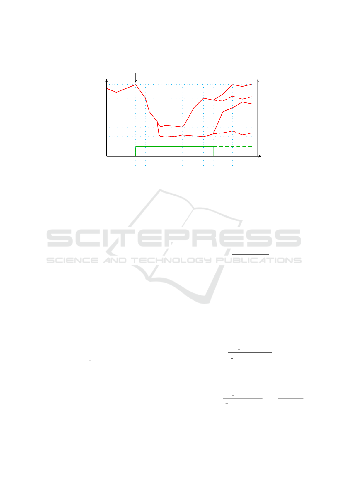
In Figure 1, we show an exemplary typical util-

ity function U (t). In the beginning, U is at the target

value U

target

. At time t

, a disturbance of strength z

happens (displayed in green) and the utility (red) de-

creases. Once it drops below the acceptance threshold

acc

at t

, a control mechanism (CM) starts to inter-

vene. At t

low

, U reaches U

low,perm

without an effective

recovery mechanism and U

low,cm

if a control mecha-

nism is acting against the impact of the disturbance.

With a CM, U starts to recover at t

rec

and passes U

acc

at t

acc

. However, without a CM, U does not recover.

We can differentiate between two classes of be-

haviour during an attack:

1) An effective CM is started and the system recov-

ers to at least U

acc

2) The system does not recover during attack (or dur-

ing a disturbance).

Furthermore, we see two different types of be-

haviour when the attack ends at t

. Either (a) the util-

ity reaches the same value as before the attack (here

target

at t

target

; solid red line in Figure 1), or (b) it

stays at the same level as during the attack (dashed

line). In total, this results in four different stereotypes

of behaviour:

1a) The system S recovers during the attack to U ≥

acc

and returns to U ≥ U

target

when the attack

ends. This is a strongly robust system.

ICAART 2017 - 9th International Conference on Agents and Artiﬁcial Intelligence

low,perm

low,cm

target

acc

low

rec

acc

¯z

target

Figure 1: Utility degradation over time. At t

a disturbance with strength z occurs. The utility U drops. When it reaches U

acc

(i.e. a utility value that is mapped on the acceptance space of the considered system, see Schmeck et al. (2010)), a control

mechanism (CM) is activated for (1) which only decreases to U

low,cm

(i.e. the lowest utility value under presence of the control

mechanism CM). At t

rec

, recovery starts and (1) passes U

acc

at t

acc

. For (2) no CM is activated and utility drops to U

low,perm

(with perm referring to a system-inherent permanent robustness level) and no recovery occurs. When the attack ends (a), the

utility recovers U

target

eventually (i.e. it reaches the target space again, see Schmeck et al. (2010)). If the attack prevails or did

permanent damage to the system (b), utility may stay at a lower value.

1b) S recovers during the attack to U ≥ U

acc

and stays

there when the attack ends. This is a weakly robust

system.

2a) S does not recover during the attack but returns to

the previous value after the attack ends. Such a

system shows just a certain "elasticity", we call it

partially robust.

2b) S does not recover during the attack, it stays at the

low utility level U

low,perm

. Such a system is not

robust at all.

While important, this only serves as a classiﬁca-

tion of different typical behaviours. However, to com-

pare the effect of different disturbances z or different

CMs, we have to quantify the utility degradation. We

deﬁne the utility degradation D

as the area between

a baseline utility (U

baseline

) and U (t) for the time when

U ≤ Uacc (see Equation 1):

(

baseline

(t) −U (t)

)

dt (1)

First, we need to deﬁne a baseline U

baseline

for the

measurement. This can be either hypothetical by us-

ing U

target

or U

acc

(in Figure 1) or we can run a refer-

ence experiment (as we will show later in Scenario 2,

see Section 4). In order to maximise the system ro-

bustness, we have to minimise D

. A system, which

never drops below U

baseline

apparently has maximal

robustness. We deﬁne the robustness during attack R

as:

U (t) dt

baseline

(t) dt

For each CM to be compared, we measure a util-

ity degradation D

. This allows comparing the be-

haviour of two CMs during an attack (such as cases

(1) and (2) from above) or the effectiveness of one

CM for different attacks.

Furthermore, when the attack ended, we can mea-

sure the long-term utility degradation D

U,long_term

which is the area between U

baseline

and the actual U for

the time after t

. This allows us to compare the cases

(1a/2a) and (1b/2b) from above. Hence, the long-term

robustness R

is deﬁned as:

target

U (t) dt

target

baseline

(t) dt

In cases where U (t) never reaches U

target

again, t

target

is ∞ (also U

is ∞) but we can calculate the open in-

tegral:

target

= ∞ → R

target

U (t) dt

target

baseline

(t) dt

= lim

t→∞

U (∞)

baseline

(∞)

In all normal cases, R is assumed to be in the in-

terval [0, 1]. It can never be negative and will only

Quantitative Robustness â

A¸S A Generalised Approach to Compare the Impact of Disturbances in Self-organising Systems

be larger than 1 if U (t) improves through the distur-

bance which happens only under very speciﬁc condi-

tions (i.e. the system settled in a local optimum before

the disturbance occurs, and is able to leave this local

optimum as a result of the CM’s intervention). Even

if the utility U (t) never recovers, we get an asymp-

totic robustness value. However, values of R

with

target

= ∞ are not comparable to values for R

with

target

, ∞ because the open integral would be always

1 in this case.

2.3 Related Work

The term “robustness” is widely used with differ-

ent meanings in literature, mostly depending on the

particular context or underlying research initiative.

Typical deﬁnitions include the ability of a system

to maintain its functionality even in the presence of

changes in their internal structure or external envi-

ronment (sometimes also called resilient or depend-

able systems) Callaway et al. (2000), or the degree to

which a system is insensitive to effects that have not

been explicitly considered in the design Slotine et al.

(1991).

When especially considering engineering of in-

formation and communication technology-driven so-

lutions, the term “robust” typically refers to a ba-

sic design concept that allows the system to func-

tion correctly (or, at the very minimum, not failing

completely) under a large range of conditions or dis-

turbances. This also includes dealing with manufac-

turing tolerances. Due to this wide scope of related

work, the corresponding literature is immense, which

is e.g. expressed by detailed reports that range back

to the 90ies Taguchi (1993). For instance, in the con-

text of scheduling systems, robustness of a schedule

refers to its capability to be executable – and leading

to satisfying results despite changes in the environ-

ment conditions Scholl et al. (2000). In contrast, the

systems we are interested in (i.e. self-adaptive and

self-organising OC systems) typically deﬁne robust-

ness in terms of fault tolerance (e.g. Jalote (1994)).

In computer networks, robustness is often used as

a concept to describe how well a set of service level

agreements are satisﬁed. For instance, Menasce et al.

explicitly investigate the robustness of a web server

controller in terms of workloads that exhibit some

sort of high variability in their intensity and/or ser-

vice demands at the different resources Menascé et al.

(2005).

More speciﬁcally and beyond these general deﬁni-

tions of the notion of robustness, we shift the focus to-

wards quantiﬁcation attempts. Only a few approaches

known in literature aim at a generalised method to

quantify robustness; in a majority of cases, self-

organised systems are either shown to perform better

(i.e. achieve a better system-inherent utility function)

or react better in speciﬁc cases (or in the presence

of certain disturbances), see e.g. ICAC (2015) and

SASO (2015). . In the following, we discuss the most

important approaches to robustness quantiﬁcation.

In the context of OC, a ﬁrst concept for a classiﬁ-

cation method has been presented in Schmeck et al.

(2010). Here, the idea is (as in our approach) to

take the system utility into account. Based on a pre-

deﬁned separation of different classes of goal achieve-

ment (i.e. distinguishing between target, acceptance,

survival, and dead spaces in a state space model of

the system S), the corresponding states are assigned to

different degrees of robustness. Consequently, differ-

ent systems are either strongly robust (i.e. not leaving

the target space), robust (i.e. not leaving the accep-

tance space), or weakly robust (i.e. returning from

the survival space in a deﬁned interval). In contrast

to our method, a quantitative comparison is not pos-

sible. In particular, this robustness classiﬁcation does

not take the recovery time into account.

Closely related is the approach by Nafz et al. pre-

sented in Nafz et al. (2011), where the internal self-

adaptation mechanism of each element in a superior

self-organising system has the goal to keep the ele-

ment’s behaviour within a pre-deﬁned corridor of ac-

ceptable states. Using this formal idea, robustness can

be estimated by the resulting goal violations at run-

time. Given that system elements have to obey the

same corridors, this would also result in a compara-

ble metric. Recently, the underlying concept has been

taken up again to develop a generalised approach for

testing self-organised systems, where the behaviour

of the system under test has to be expressable quanti-

tatively Eberhardinger et al. (2015). However, this de-

pends on the underlying state variables and invariants

that are considered – which might be more difﬁcult to

assess at application level (compared to considering

the utility function in our approach).

In contrast, Holzer et al. nodes are considered

as stochastic automaton in a network and model the

nodes’ conﬁguration as a random variable Holzer and

de Meer (2011). Based on this approach, they com-

pute the level of resilience (the term is used there sim-

ilarly to robustness in this paper) depending on the

network’s correct functioning in the presence of mal-

functioning nodes that are again modelled as stochas-

tic automatons Holzer and de Meer (2009). In con-

trast to our approach, this does not result in a compa-

rable metric and limits the scope of applicability due

to the underlying modelling technique.

From a multi-agent perspective, Di Marzo Seru-

ICAART 2017 - 9th International Conference on Agents and Artiﬁcial Intelligence

gendo approached a quantiﬁcation of robustness us-

ing the accessible system properties Di Marzo Seru-

gendo (2009). In general, properties are assumed to

consists of invariants, robustness attributes, and de-

pendability attributes. By counting or estimating the

conﬁguration variability of the robustness attributes,

systems can be compared with respect to robustness.

Albeit the authors discuss an interesting general idea,

a detailed metric is still open.

Also in the context of multi-agent systems, Nimis

and Lockemann presented an approach based on

transactions Nimis and Lockemann (2004). They

model a multi-agent system as a layered architecture

(i.e. seven layers from communication at the bot-

tom to the user at the top layer). Of particular in-

terest is the third layer, i.e. the conversation layer.

The key idea of their approach is to treat agent con-

versations as distributed transactions. The system is

then assumed to be robust, if guarantees regarding

these transactions can be formulated. This requires

technical prerequisites, i.e. the states of the partici-

pating agents and the environment must be stored in

a database – this serves as basis for formulating the

guarantees. Obviously, such a concept assumes hard

requirements that are seldom available, especially not

in open, distributed systems where system elements

are not under control of a centralised element and

might behave unpredictably.

To conclude this discussion, we can observe that a

generalised approach to quantify robustness is needed

that: (a) works on externally measurable values, (b)

does not need additional information sources (e.g.

transactional data-bases), (c) distinguishes between

system-inherent (or passive) and system-added (or ac-

tive) robustness (to allow for an estimation of the

effectiveness of the particular mechanism) and (d)

comes up with a measure that allows for a comparison

of different systems for the same problem instance.

We claim that our approach as outlined before fulﬁls

all of these aspects. In order to demonstrate the effec-

tiveness, we apply it to three different use cases in the

following part of this paper.

3 APPLICATION SCENARIO 1:

WIRELESS SENSOR

NETWORKS

Wireless Sensor Networks (WSNs) consist of spa-

tially distributed nodes which communicate over a ra-

dio interface. Nodes sense locally and send the result

to the root node in the network. Since most nodes

cannot reach root directly, other nodes have to relay

packets. To ﬁnd a path to root, the Routing Proto-

col for Lossy and Low Power Networks (RPL) (Win-

ter et al., 2012) is used. The primary objective (O1)

in such networks is to reach a high Packet Delivery

Rate (PDR; ranges from 0 to 1). Since nodes are

battery-powered, the secondary objective (O2) is to

minimise the number of Transmitted Packets (#TX)

because sending data over the air causes most power

consumption in WSNs. These two objectives translate

into two utility functions, which we have to investi-

gate with respect to their robustness. Utility function

1 is PDR(t), utility function 2 is #TX(t).

In open distributed sensor networks, attacks by

malicious or broken nodes can occur, which lead to

poor PDR. To counter such threats, we introduced

end-to-end trust in RPL in previous work (Kantert

et al., 2016b). In this trust-enhanced approach, the

nodes assess the trustworthiness of their parents and

isolate bad-behaving nodes. This constitutes a spe-

ciﬁc self-organised control mechanism CM. We are

interested in a comparison of different variants of

CMs:

CM0 OF0. This is the default routing mechanism

in RPL as described in (Winter et al., 2012).

It selects parents by the smallest rank.

CM1 Trust + ETX. Nodes use a trust metric

to rate and isolate bad-performing parents.

See (Kantert et al., 2016b) for more details.

The particular method is not of interest in

the context of this paper, it serves as a repre-

sentative for a more powerful, self-organised

control mechanism.

CM2 Trust + ETX + Second Chance. This ap-

proach is similar to the previous one but

also incorporates a mechanism to retry pre-

viously isolated parents occasionally (i.e. af-

ter re-stabilising the system, see again (Kan-

tert et al., 2016b) for details). This approach

serves as a representative with even more de-

cision freedom of the CM.

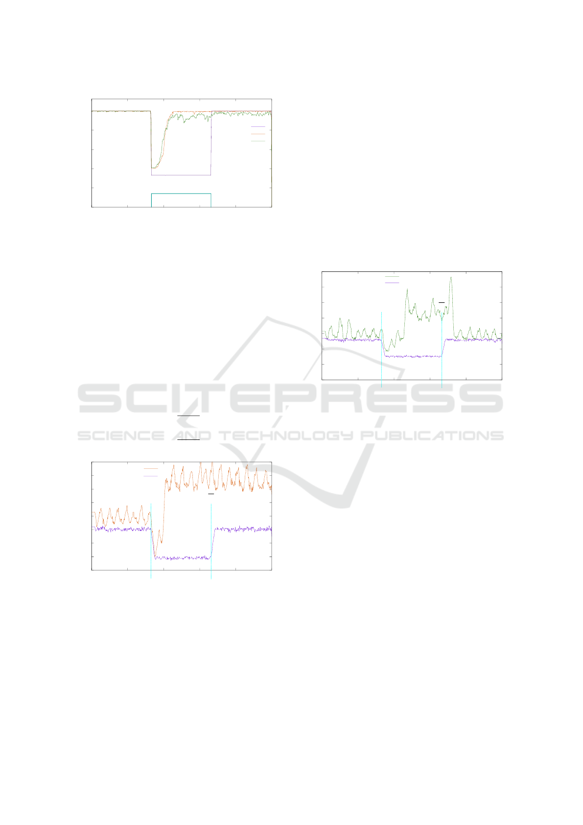
In an undisturbed RPL network, our trust-

enhanced system implemented as CM1 behaves very

similar to standard RPL (CM0). However, when an

attack occurs, standard RPL looses numerous pack-

ets and PDR drops because it cannot handle (inten-

tional or unintentional) malicious behaviour. When

enabling our approach, nodes start to identify and iso-

late bad-behaving parents. Hence, the PDR recovers

to nearly 100% (i.e. U

target

) while the attack happens.

Standard RPL only recovers after the attack ends (see

Figure 2).

For O1 (PDR(t)), D

is 112 for CM0, 13.7 for

CM1 and 17.9 for CM2. Quantitatively, D

of CM1

Quantitative Robustness â

A¸S A Generalised Approach to Compare the Impact of Disturbances in Self-organising Systems

0.2

0.4

0.6

0.8

0 100 200 300 400 500

TRUST + ETX

OF0

TRUST + ETX + SC

Figure 2: Objective 1, Utility function 1: Packet Delivery

Rate (PDR) over sequences (time). At time step 160, an at-

tack starts and ends at time step 340. PDR drops to about

30% for OF0 during the attack and recovers afterwards.

TRUST + ETX and TRUST + ETX + Second-Chance re-

cover during the attack and stay near 100% PDR until the

end of the experiment.

is 87.7% better than CM0 and CM2 is 84% better than

CM0. Also, CM1 has 23.5% smaller D

than CM2.

The baseline is 1 (see Equation 2). R

for CM0 has

a value of 70% (3), CM1 has a value of 91% (4) and

CM2 has a value of 89%(5).

baseline

(t) B 1 (2)

a,CM0

≈ 70% (3)

a,CM1

146.3

160

≈ 91% (4)

a,CM2

142.1

160

≈ 89% (5)

100

110

120

0 100 200 300 400 500

TRUST + ETX

OF0

Figure 3: Objective 2, Utility function 2: Transmitted Pack-

ets (#TX) over time. At time step 160, an attack starts, and

ends it at time step 340. During the attack #TX increases

for the TRUST + ETX control mechanism (CM1) and stays

at that level after the attack. For OF0 (CM0), #TX drops

during the attack and recovers to the undisturbed level af-

terwards.

For objective O1 (i.e. PDR(t)) CM1 recovers per-

fectly during the attack and returns to the same value

as before the attack. Therefore, in this scenario, RPL

with Trust + ETX is rated as strongly robust. How-

ever, this changes when we look at the second ob-

jective O2 represented by utility function 2: metric

#TX(t) (the number of transmitted packets, see Fig-

ure 3). When the attack starts, #TX drops for all CMs

(which would be perfect if PDR stayed at a constant

level). For Trust + ETX it increases to a higher level

because the new routes are longer and require more

transmissions. This is expected since some parents

failed. However, after the attack ends, only standard

RPL returns to its previous #TX. Trust + ETX stays

at a high level. This is acceptable when dealing with

intentional malicious attackers but this is bad when

disturbances are only temporary. Therefore, Trust +

ETX is not robust regarding the second utility func-

tion.

100

120

140

160

0 100 200 300 400 500

TRUST + ETX + SC

OF0

Figure 4: Objective 2, Utility function 2: Transmitted Pack-

ets (#TX) over time. At time step 160, an attack starts, and

ends at time step 340. During the attack #TX(t) increases

for the TRUST + ETX + Second-Chance (CM2). For OF0

(CM0), #TX(t) drops during the attack and recovers to the

same level as before afterwards. Unlike in Figure 3, TRUST

+ ETX + Second-Chance (CM2) recovers to a similar level

as before the attack.

Most energy in wireless sensor nodes is used when

sending packets. Thus, to recover the energy con-

sumption and #TX after an attack, we introduced

TRUST + ETX + Second-Chance as a third control

mechanism CM2 which retries parents when the sys-

tem has stabilised (from a node’s local perspective).

This leads to a slight decrease of the PDR during the

attack because nodes loose packets when retrying dur-

ing an attack. However, after the attack the PDR is

very similar and #TX recovers to its level from before

the attack (see Figures 2 and 4).

For O2, we measure D

only after the attack.

Quantitatively, D

for CM1 is ∞ because it does not

return to the previous values. For CM0 D

is about

0. CM2 needs some time to recover and has a D

of 1998.6. Thus, CM0 is the best metric when only

considering O2 (since it is very bad for O1). In our

robustness metric, we have to assume that a higher

utility is better. In this case, the best utility for O2

would be a value of 0 (which is unrealistic). There-

ICAART 2017 - 9th International Conference on Agents and Artiﬁcial Intelligence

fore, we invert U (t) to get a utility function for the

calculation of R

(see Equation 6). This results in a

baseline U

baseline

of 43 (saved packets per second; see

Equation 7). For CM1 this results in an asymptotic

long-term robustness R

of 35% (8). CM2 recovers

and has a robustness value R

of 47% (not compara-

ble to CM1; Equation 9).

normalised

(t) B 120 −U (t) (6)

baseline

B 120 − 77 = 43

packets

(7)

l,CM1

≈

120 − 105

≈ 35% (8)

l,CM2

≈

401.4

860

≈ 47% (9)

CM2 (TRUST + ETX + Second-Chance) is

strongly robust for PDR. Also, it is robust regarding

#TX. It does not recover during the attack (because

better routes do not exist) but it recovers to the previ-

ous state when the attack ends.

4 APPLICATION SCENARIO 2:

OPEN DISTRIBUTED SYSTEMS

Another scenario we measured robustness in is the

simulation of an open, distributed Multi-agent Sys-

tem with applied trust metrics, the Trusted Desktop

Grid (TDG) (Edenhofer et al., 2015). In this grid,

jobs J are created by the agents and split into work

units (WU), which are calculated in a distributed way

by the agents. The success (or utility) is expressed

as the speedup σ(t). σ(t) is deﬁned as the time the

agent would have needed to process all work units on

its own (sel f ) divided by the real time it took to cal-

culate the job in a distributed way in the system (dist),

see Equation 10. A job J is released in time step t

rel

and completed in t

compl

σ =

∑

compl

sel f

− t

rel

sel f

)

∑

compl

dist

− t

rel

dist

)

(10)

In this scenario, our objective is to maximise

the utility function speedup σ(t) (see Equation 10).

Nodes make decisions based on a local trust met-

ric and isolate bad-behaving agents using this Con-

trol Mechanism (CM1; see (Klejnowski, 2014) for de-

tails). We compare different attacks:

A0 No attack. Used as baseline.

A1 A short attack which ends at t

Figure 5: Disturbance D1: Robustness in the TDG. Attack

of 100 EGO from tick 80,000 to 120,000 and continuous

from 80,0000 (A2). t

low

marks the point in time, where σ(t)

is at its lowest. The speedup starts to recover (t

rec

) during

the attack until it reaches U

acc

(at t

acc

). After the attack has

stopped, the speedup returns to the level it had before for

A1. However, it stays at about 10 for A2.

A2 Permanent attack which continues until the ex-

periment ends.

Additionally, we consider two different disturbances

by stereo-type attacker behaviour:

D1 Egoistic agents (EGO) are accepting all WU,

but abort 80% of them after some time, which

decreases σ(t) because these WUs have to be

redistributed.

D2 Freeriding agents (FRE) do not accept WU at

all. They reject WUs right away but try to dis-

tribute their WUs at the same time.

For evaluation purposes, we investigated exem-

plary scenarios that incorporate disturbed system

states. More precisely, we simulated 100 well-

behaving adaptive agents (ADA). At time t

, 100 bad-

behaving egoistic agents (EGO; D1) join the system,

simulating a colluding attack. To show the effect of

robustness in the system, we calculated the average

speedup of 10 runs with a length of 200,000 ticks

each. We want to compare the system behaviour (i.e.

its robustness) under two different attacks. Attack

A1 starts at tick 80,000 and lasts 40,000 ticks. At-

tack A2 is a continuous attack of 100 EGO starting at

tick 80,000. As baseline, we ran the same experiment

without an attack (A1; see Figure 5).

In both attacks (A1 and A2), the average speedup

of the ADA during the attack of the EGO is decreased,

due to the malevolent behaviour of the EGO. t

low

marks the point in time, where σ of the ADA is at its

lowest. During the attack, once the average speedup

of ADA increases by 5% (t

rec

) over σ(t) at t

low

, the re-

covery phase is said to start; recovery is deﬁned to be

reached, if σ(t) is at least 75% (at t

acc

) of σ(t) before

the attack in t

In the ﬁrst attack, after tick 120,000, the ADA

have to redistribute the WUs formerly occupied by

Quantitative Robustness â

A¸S A Generalised Approach to Compare the Impact of Disturbances in Self-organising Systems

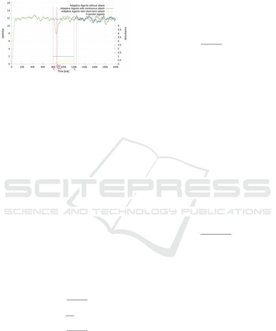
Figure 6: Disturbance D2: Robustness in the TDG. Attack

of 100 FRE from tick 80,000 to 120,000 (A1) and continu-

ous from 80,0000 (A2) t

low

marks the point in time, where

σ(t) is at its lowest. The speedup starts to recover (t

rec

)

during the attack and quickly reaches U

acc

and U

target

for

both A1 and A2. At tick 120,000 A1 and A2 are the same

because the attackers are fully isolated and have no further

inﬂuence.

EGO. After these WUs have been successfully cal-

culated, σ(t) recovers to the level it had before the at-

tack. In both attacks, σ (t) of the ADA recovers during

the attack until it reaches the acceptance space (i.e.

system states where the utility is above U

acc

). This

is due to the EGOs getting low trust ratings because

they abort their assigned WUs. Yet, they manage to

retain a high enough reputation to still get some WUs

computed by other agents. As 80% of the WUs held

by EGOs have to be redistributed, σ(t) of the ADA

cannot recover to the level it had before the attack.

Quantitatively, D

is 130,105 below the baseline

for both A1 and A2. After the attack, D

is 6250

for A2. D1 has a permanent inﬂuence and CM1 is

not able to fully mitigate the effect. We measured the

baseline utility U

baseline

in a reference experiment. R

for A1 and A2 is with 72% (see Equation 11). Similar

to, O2 in Scenario 1, only A2 fully recovers. For A1,

we calculate R

in an open integral in Equation 12.

Again, not comparable, R

for A2 can be calculated in

a closed integral (see Equation 13; the open integral

would have a value of 1).

a,A1

= R

a,A2

349, 895

480, 000

≈ 73% (11)

l,A1

≈

9.5

≈ 79% (12)

l,A2

113, 750

120, 000

≈ 95% (13)

Similarly, we run experiments for disturbance D2

with free-riding agents (see Figure 6). Since those

agents are simpler to detect, they are isolated within

the attack period of A1 and the system fully recovers

to U

target

within the attack. U

is 13, 056 for both A1

and A2 during the attack. After the attack ends, A1 is

already fully recovered and the utility for A1 and A2

is similar. CM1 is able to fully mitigate this distur-

bance D2. R

is 97% (see Equation 14). Since U (t)

fully recovers for both attacks, R

is about 100% for

A1 and A2.

a,D2

466, 944

480, 000

≈ 97% (14)

5 APPLICATION SCENARIO 3:

URBAN TRAFFIC

MANAGEMENT

A third scenario that is often used as basis to inves-

tigate a self-organisation mechanism due its inherent

dynamics and distributed nature is the control of traf-

ﬁc lights in urban areas, see (Bazzan and Klügl, 2009;

Dinopoulou et al., 2006) for instance. One of the ma-

jor OC-based contributions in this context is the Or-

ganic Trafﬁc Control (OTC) system (Prothmann et al.,

2011) that applies the observer/controller approach as

well as an autonomous and safety-oriented learning

process to the trafﬁc domain.

In OTC, each intersection of the inner-city road

network is managed by an observer/controller in-

stance that gathers detector data about the underly-

ing trafﬁc conditions (in terms of ﬂows passing each

turning movement) and reacts by adapting green dura-

tions. The success of the control strategy is typically

expressed as ﬂow-weighted delays:

∑

× t

d,i

)

∑

(15)

Where M

corresponds to the current trafﬁc ﬂow at the

i-th turning of the observed intersection and t

d,i

de-

notes the average waiting time with respect to a single

turning t

. This metric is also referred to as Level of

Service (LoS) Transportation Research Board (2000).

In addition, the same metric is used to determine the

most promising progressive signal system Tomforde

et al. (2010).

Adapting trafﬁc signalisation to changing de-

mands and coordinating intersection controllers pro-

vides a ﬁrst step towards robustness – but this does

not dissolve the initial disturbance. In terms of the

previously developed notion, this accounts as pas-

sive robustness. Re-routing of trafﬁc participants

counters the disturbance (i.e. a blocked road or

trafﬁc jams) directly and can be considered as ac-

tive robustness mechanism in this context. In pre-

vious work, we equipped OTC with such a mecha-

nism Prothmann et al. (2012). Based on ideas re-

sembling the Link State or Distance Vector Routing

ICAART 2017 - 9th International Conference on Agents and Artiﬁcial Intelligence

protocols as known from the computer networks do-

main(Tanenbaum, 2002), information about the short-

est routes are exchanged between intersection con-

trollers and provided to drivers at each incoming inter-

section, see Prothmann et al. (2011, 2012) for details.

54 H. Prothmann et al.

currently best paths to all destinations are known and can be stored in the

routing tables that are associated with the intersection approaches. Like for the

DVR protocol, the table entries contain the destination, the recommended next

turning, and the estimated travel time to the destination.

5 Evaluation

To evaluate the potential beneﬁts of a DRG system, OTC-controlled intersections

with and without their RCs have been compared in a simulation study.

5.1 Experimental Setup

Fig. 1. Network map (incl. incident location)

The evaluation has been con-

ducted for a simulated network

that is illustrated in Fig. 1.

The network consists of three

Manhattan-type sub-networks. It

contains 27 signalised intersec-

tions (depicted as circles) and

28 prominent destinations (de-

picted as diamonds). Within each

sub-network, the intersections are

connected by one-laned road seg-

ments of 250 mlengththatpro-

vide two additional turning lanes

starting 100 m before an intersection. Regions are connected by two-laned roads.

Signalised intersections are operated by an observer/controller (see Sect. 3)

and can provide route recommendations for the prominent destinations. Each

destination also serves as origin for traﬃc entering the network. Two scenarios

are investigated:

– In the regular scenario, eight vehicles per hour travel from every origin to

every destination. In total, 6048 vehicles traverse the network in every hour.

Since this demand does not cause signiﬁcant jams at the network’s intersec-

tions, the scenario allows to evaluate the impact of DRG under uncongested

conditions. It is simulated for a period of three hours.

– In the incident scenario, the same amount of traﬃc traverses the network.

However, one of the roads connecting two sub-networks is temporarily blocked

due to an incident (see Fig. 1). The blockage aﬀects both directions of the

road, occurs after 15 minutes and lasts for 20 minutes within the two hour

simulation period. The incident scenario allows to evaluate the beneﬁt of

DRG in the presence of disturbances.

As the literature reports a widely varying driver acceptance for VMS-based

route recommendations [4, 5], acceptance rates of 0.125 (low), 0.375 (medium),

Figure 7: An exemplary model of 27 intersections (depicted

as grey circles), forming three connected Manhattan-style

road networks. Trafﬁc enters and leaves the network at lo-

cations referred to as destinations (depicted as light-grey di-

amonds). In the evaluation, the red road is blocked during

attack A1.

In this scenario, the objective is to maximise the

utility function trafﬁc ﬂow which can be measured

globally. At t

, one road is blocked until t

(attack

A1, red road in Figure 7). We compare three different

control mechanisms:

CM0 No active control mechanism. Used as base-

line.

CM1 OTC without routing.

CM2 OTC with routing.

The evaluation has been conducted for a simu-

lated network that is illustrated in Figure 7. The net-

work consists of three Manhattan-type sub-networks.

It contains 27 signaled intersections (depicted as cir-

cles) and 28 prominent destinations (depicted as dia-

monds). Within each sub-network, the intersections

are connected by one-laned road segments of 250m

length that provide two additional turning lanes start-

ing 100m before an intersection. Regions are con-

nected by two-laned roads. Signalised intersections

are operated by an observer/controller (i.e. OTC) and

can provide route recommendations for the prominent

destinations. Each destination also serves as origin for

trafﬁc entering the network.

We conﬁgured the simulation as follows: eight

vehicles per hour travel from every origin to every

destination. Since this demand does not cause sig-

niﬁcant jams at the network’s intersections, the sce-

nario allows evaluating the impact of routing mecha-

nisms under uncongested conditions. As disturbance,

we temporarily blocked one of the roads connecting

two sub-networks due to an incident (see mark in

Figure 7). The blockage affects both directions of

the road, occurs after 25 min and lasts for 40 min

within the simulation period. The incident scenario

allows analysing the impact of the two different adap-

tation mechanisms (CM1 = OTC without routing, and

CM2 = OTC with routing) in comparison to a stan-

dard ﬁxed-time control approach (= CM0).

Within the professional simulator Aimsun Barceló

et al. (2005), we performed ﬁve runs of experiments

for each instance under evaluation and computed av-

erages. Figure 8 depicts the achieved results. We can

clearly observe that the typical system behaviour of

a disturbed and recovering system is visible in this

scenario. When considering the OTC system without

routing in comparison to a standard ﬁxed-time con-

trol, we can distinguish two effects: a) the ﬁxed-time

controller (i.e. CM0) deﬁnes the base-line (i.e. the

maximum loss of utility) and b) the standard OTC sys-

tem (CM1) already provides a permanent robustness

increase that improves the behaviour even if no dis-

turbance takes place. If activating the routing mech-

anism (CM2), an active robustness is added. Quan-

titatively, U

for CM1 is about 5.4% better than the

reference solution (CM0) (i.e. 5534 vs 5250 vehicles

per hour) and routing (CM2) adds further utility, i.e.

an improvement in U

of 14.0% (i.e. 6312 vehicles

per hour).

baseline

(t) B 7, 000

vehices

= 116.7

vehicles

min

(16)

a,CM0

87.5

116.7

≈ 75% (17)

a,CM1

92.2

116.7

≈ 79% (18)

a,CM2

105.2

116.7

≈ 90% (19)

To calculate the robustness, we use a baseline based

on U

target

(see Equation 16). Using the U

values from

above, we calculate the robustness R

for all CMs in

Equations (17) to (19). What we can see in the ﬁg-

ure is that a passive robustness is already in place

with CM0, since most of the network is still operat-

ing without strong impact of the disturbance (in terms

of trafﬁc ﬂow through the network). This changes

if we just consider the blocked link: Here, for all

three mechanisms the utility drops to zero and recov-

ers immediately when the blockade is removed (not

shown in ﬁgure). Hence, the robustness is achieved

at network-level, since participants are routed using

the best available link (i.e. with routing mechanism,

CM2) or at least the non-affected participants beneﬁt

due to longer green durations (i.e. a blocked road re-

ceives a lower fraction of the phase cycle time when

using OTC, CM1 and CM2). With this mechanism

at hand, we are now able to compare the developed

Quantitative Robustness â

A¸S A Generalised Approach to Compare the Impact of Disturbances in Self-organising Systems

1000

2000

3000

4000

5000

6000

7000

8000

time in min

Utility: Traffic flow in veh/h

Fixed-time Control OTC w/o routing OTC w/ routing

𝑡

𝑧

𝑡

𝑧

𝑡

𝑎𝑐𝑐

(for )

𝑡

𝑙𝑜𝑤

𝑈

𝑎𝑐𝑐

Figure 8: Utility over time for OTC. At t

one road is blocked (attack A1) and trafﬁc has to be redirected. With ﬁxed-

time control (CM0), utility drops by nearly 3,000 vehicles per hour. OTC without routing (CM1) performs slightly better.

Compared, OTC with routing (CM2) only drops about 1,000 vehicles per hour. After the attack A1 ends, all CMs recover the

system to their previous utility.

mechanisms to other solutions from the state-of-the-

art (such as Wedde et al. (2007) for self-organised

routing or Dinopoulou et al. (2006) for autonomous

trafﬁc controllers) and quantify the varying robust-

ness levels in different disturbance scenarios.

6 DISCUSSION

We demonstrated that our approach is applicable to

three varying scenarios from different application do-

mains. In Scenario 1, we compared three different

control mechanisms with two different objective func-

tions for wireless sensor networks. The resulting val-

ues are reasonable and allow for a simple and effec-

tive comparison of robustness levels for the consid-

ered CMs. In Scenario 2, we compared two different

attack types and two different disturbances in a grid

scenario. We measured the long-term inﬂuence for

the disturbances and found that only one of the dis-

turbances has a permanent effect. Afterwards, in Sce-

nario 3, we measured the robustness for three CMs in

a trafﬁc management scenario.

The general shape of the utility graph was very

similar in all our scenarios. Still, the utility degrada-

tion U

is not comparable between scenarios because

it has an application speciﬁc unit (i.e. it is hard to

compare apples and oranges). However, our robust-

ness metrics R

and R

are unit free and always have

the same boundaries. Thus, they allow some compar-

ison between different systems.

Nevertheless, some limitations apply: We have to

set a ﬁxed attack length t

− t

. This limits the appli-

cability of the concepts to those cases where a distur-

bance is observable in the ﬁrst place. Current research

addresses this topic by developing techniques to deal

with this issue. Also, it inﬂuences the value of R as

illustrated by Scenario 2. If we had set t

, earlier the

robustness R

for both CMs would be lower. A simi-

lar challenge occurs when calculating R

for two CMs

which reach U

target

at different times. To make their

robustness R

values comparable, a later t

target

has to

be chosen. This issue can be solved but it requires

some caution when designing experiments.

We noticed another challenge when calculating R

for O2 in Scenario 1 because our goal was to minimise

the metric. However, for a utility function U (t) a

higher value should be better. Hence, we had to invert

the objective function to calculate the utility. There

is no need to normalise the utility function but larger

values must be better which is important to keep the

robustness values inside the interval between 0 and 1.

Finally, we saw in Scenario 1 that it is crucial to

choose the right utility function. If we only consider

O1, A1 has the best robustness. However, if we also

take into account O2, A2 is clearly better. The re-

maining challenge here is to properly combine multi-

ple metrics.

In future work, we will focus on quantitatively

comparing similar mechanisms in different applica-

tion scenarios. Also, we would like to extend the se-

lection of integration limits for better comparison.

7 CONCLUSION

Self-adaptation and self-organisation are concepts in-

creasingly incorporated in system design. This is

ICAART 2017 - 9th International Conference on Agents and Artiﬁcial Intelligence

mostly due to one key motivation: We want to im-

prove the robustness of technical systems in terms of

a utility preservation in order to maintain the system’s

functionality even under harsh external conditions or

the presence of internal failures (we refer to such ef-

fects in general as disturbances). Hence, one of the

most important aspects to judge whether one speciﬁc

solution is more beneﬁcial than another is to estimate

which system is more robust. Such a decision process

needs a quantitative basis to come up with a mean-

ingful statement. In this paper, we presented a novel

method that estimates such a measurement at runtime.

We discussed the state-of-the-art and explained

that existing approaches have drawbacks, e.g. requir-

ing too much internal information, measuring only

certain aspects (such as the time), being application-

speciﬁc, or abstracting the robustness too far (i.e.

coming up with a discretisation of a few classes only).

With our method, we focus on externally measurable

attributes only and allow for a generalised concept

for comparing robustness. We further distinguish be-

tween a permanent part of robustness that is system

inherent and a part that is generated by internal adap-

tation mechanisms. We demonstrated the expressive-

ness of the developed approach in terms of three case

studies, i.e. from the desktop grid, the wireless sensor

network, and the trafﬁc control domains.

In future work, we will investigate how our

method behaves when comparing different systems

within the same application domain. In addition,

we focus on questions regarding the heterogeneity

of occurring disturbances: Where are the drawbacks

and advantages of the developed technique and what

needs to be improved to come up with a fully gener-

ally applicable method?

REFERENCES

(2015). 2015 IEEE 9th International Conference on Self-

Adaptive and Self-Organizing Systems, Cambridge,

MA, USA, September 21-25, 2015. IEEE Computer

Society.

(2015). 2015 IEEE International Conference on Autonomic

Computing, Grenoble, France, July 7-10, 2015. IEEE

Computer Society.

Barceló, J., Codina, E., Casas, J., Ferrer, J., and García, D.

(2005). Microscopic trafﬁc simulation: A tool for the

design, analysis and evaluation of intelligent transport

systems. Journal of Intelligent and Robotic Systems,

41(2–3):173–203.

Bazzan, A. L. C. and Klügl, F., editors (2009). Multi-Agent

Systems for Trafﬁc and Transportation Engineering.

Idea Group Publishing, Hershey, PA, US.

Callaway, D. S., Newman, M. E., Strogatz, S. H., and Watts,

D. J. (2000). Network robustness and fragility: Per-

colation on random graphs. Physical review letters,

85(25):5468.

Choi, S., Buyya, R., Kim, H., and Byun, E. (2008). A

Taxonomy of Desktop Grids and its Mapping to State

of the Art Systems. Technical report, Grid Comput-

ing and Dist. Sys. Laboratory, The University of Mel-

bourne.

Di Marzo Serugendo, G. (2009). Stabilization, Safety, and

Security of Distributed Systems: 11th International

Symposium, SSS 2009, Lyon, France, November 3-6,

2009. Proceedings, chapter Robustness and Depend-

ability of Self-Organizing Systems - A Safety Engi-

neering Perspective, pages 254–268. Springer Berlin

Heidelberg, Berlin, Heidelberg.

Dinopoulou, V., Diakaki, C., and Papageorgiou, M. (2006).

Applications of the urban trafﬁc control strategy

tuc. European Journal of Operational Research,

175(3):1652–1665.

Eberhardinger, B., Anders, G., Seebach, H., Siefert, F., and

Reif, W. (2015). A research overview and evalua-

tion of performance metrics for self-organization al-

gorithms. In 2015 IEEE International Conference

on Self-Adaptive and Self-Organizing Systems Work-

shops, SASO Workshops 2015, Cambridge, MA, USA,

September 21-25, 2015, pages 122–127.

Edenhofer, S., Stifter, C., Jänen, U., Kantert, J., Tomforde,

S., Hähner, J., and Müller-Schloer, C. (2015). An

accusation-based strategy to handle undesirable be-

haviour in multi-agent systems. In 2015 IEEE Interna-

tional Conference on Autonomic Computing, Greno-

ble, France, July 7-10, 2015, pages 243–248.

Holzer, R. and de Meer, H. (2009). Quantitative model-

ing of self-organizing properties. In Self-Organizing

Systems, 4th IFIP TC 6 International Workshop, IW-

SOS 2009, Zurich, Switzerland, December 9-11, 2009.

Proceedings, pages 149–161.

Holzer, R. and de Meer, H. (2011). Methods for approxima-

tions of quantitative measures in self-organizing sys-

tems. In Self-Organizing Systems - 5th International

Workshop, IWSOS 2011, Karlsruhe, Germany, Febru-

ary 23-24. 2011. Proceedings, pages 1–15.

IBM (2005). An architectural blueprint for autonomic com-

puting. Technical report, IBM.

Jalote, P. (1994). Fault tolerance in distributed systems.

Prentice-Hall, Inc.

Kantert, J., Edenhofer, S., Tomforde, S., Hähner, J.,

and Müller-Schloer, C. (2016a). Normative Con-

trol – Controlling Open Distributed Systems with Au-

tonomous Entities, volume 7 of Autonomic Systems,

pages 87–123. Springer International Publishing.

Kantert, J., Reinhard, F., von Zengen, G., Tomforde, S.,

Wolf, L., and Müller-Schloer, C. (2016b). Combin-

ing Trust and ETX to Provide Robust Wireless Sen-

sor Networks. In Varbanescu, A. L., editor, Work-

shop Proceedings of the 29th International Confer-

ence on Architecture of Computing Systems, chap-

ter 16, pages 1–7. VDE Verlag GmbH, Berlin, Offen-

bach, DE, Nuremberg, Germany.

Klejnowski, L. (2014). Trusted Community: A Novel Mul-

tiagent Organisation for Open Distributed Systems.

PhD thesis, Leibniz Universität Hannover.

Quantitative Robustness â

A¸S A Generalised Approach to Compare the Impact of Disturbances in Self-organising Systems

Menascé, D. A., Bennani, M. N., and Ruan, H. (2005).

Self-star Properties in Complex Information Systems:

Conceptual and Practical Foundations, chapter On

the Use of Online Analytic Performance Models, in

Self-Managing and Self-Organizing Computer Sys-

tems, pages 128–142. Springer Berlin Heidelberg,

Berlin, Heidelberg.

Mnif, M. and Müller-Schloer, C. (2006). Quantitative

Emergence. In Proceedings of the 2006 IEEE Moun-

tain Workshop on Adaptive and Learning Systems

(SMCals 2006), held 24 Jul - 26 Jul 2006, Utah State

University College of Engineering Logan, UT, USA,

pages 78–84, Piscataway, NJ, USA. IEEE.

Nafz, F., Seebach, H., Steghöfer, J.-P., Anders, G., and Reif,

W. (2011). Constraining Self-organisation Through

Corridors of Correct Behaviour: The Restore In-

variant Approach. In Müller-Schloer, C., Schmeck,

H., and Ungerer, T., editors, Organic Computing –

A Paradigm Shift for Complex Systems, Autonomic

Systems, pages 79 – 93. Birkhäuser Verlag, Basel,

Switzerland.

Nimis, J. and Lockemann, P. C. (2004). Robust multi-agent

systems: The transactional conversation approach. In

First International Workshop on Safety and Security in

Multiagent Systems (SASEMAS’04), S, pages 73–84.

Prothmann, H., Tomforde, S., Branke, J., Hähner, J.,

Müller-Schloer, C., and Schmeck, H. (2011). Or-

ganic Trafﬁc Control. In Organic Computing – A

Paradigm Shift for Complex Systems, pages 431 – 446.

Birkhäuser Verlag.

Prothmann, H., Tomforde, S., Lyda, J., Branke, J., Hähner,

J., Müller-Schloer, C., and Schmeck, H. (2012). Self-

organised Routing for Road Networks . In Proc. of the

International Workshop on Self-Organising Systems

(IWSOS’12), held in Delft, The Netherlands, March

15 - 16, 2012, number 7166 in LNCS, pages 48 – 59.

Springer Verlag.

Schmeck, H., Müller-Schloer, C., Çakar, E., Mnif, M., and

Richter, U. (2010). Adaptivity and Self-organisation

in Organic Computing Systems. ACM Transactions on

Autonomous and Adaptive Systems (TAAS), 5(3):1–32.

Scholl, A. et al. (2000). Robuste planung und optimierung:

Grundlagen, konzepte und methoden; experimentelle

untersuchungen. Technical report, Darmstadt Tech-

nical University, Department of Business Administra-

tion, Economics and Law, Institute for Business Stud-

ies (BWL).

Slotine, J.-J. E., Li, W., et al. (1991). Applied nonlinear

control, volume 199. Prentice-Hall Englewood Cliffs,

NJ.

Taguchi, G. (1993). Robust technology development. Me-

chanical Engineering-CIME, 115(3):60–63.

Tanenbaum, A. S. (2002). Computer Networks. Pearson

Education, 4th edition.

Tomforde, S., Prothmann, H., Branke, J., Hähner, J., Mnif,

M., Müller-Schloer, C., Richter, U., and Schmeck, H.

(2011). Observation and Control of Organic Systems.

In Organic Computing - A Paradigm Shift for Complex

Systems, pages 325 – 338. Birkhäuser Verlag.

Tomforde, S., Prothmann, H., Branke, J., Hähner, J.,

Müller-Schloer, C., and Schmeck, H. (2010). Possi-

bilities and limitations of decentralised trafﬁc control

systems. In 2010 IEEE World Congress on Computa-

tional Intelligence (IEEE WCCI 2010), pages 3298–

3306. IEEE.

Transportation Research Board (2000). Highway capacity

manual. Technical report, National Research Council,

Washington D.C., US.

Wedde, H. F., Lehnhoff, S., et al. (2007). Highly dy-

namic and adaptive trafﬁc congestion avoidance in

real-time inspired by honey bee behavior. In Hol-

leczek, P. and Vogel-Heuser, B., editors, Mobilität und

Echtzeit – Fachtagung der GI-Fachgruppe Echtzeit-

systeme, pages 21–31. Springer.

Winter, T., Thubert, P., Brandt, A., Hui, J., Kelsey, R.,

Levis, P., Pister, K., Struik, R., Vasseur, J., and

Alexander, R. (2012). RPL: IPv6 Routing Protocol

for Low-Power and Lossy Networks. RFC 6550 (Pro-

posed Standard).

ICAART 2017 - 9th International Conference on Agents and Artiﬁcial Intelligence