
Probabilistic Background Modelling for Sports Video Segmentation
Nikolas Ladas
1
, Paris Kaimakis
2
and Yiorgos Chrysanthou
1
1
Department of Computer Science, University of Cyprus, Nicosia, Cyprus
2
Department of Computing, University of Central Lancashire Cyprus, Larnaca, Cyprus
{nladas, yiorgos}@cs.ucy.ac.cy, pkaimakis@uclan.ac.uk
Keywords:
Segmentation, Background Modelling, Shadow Detection, Visibility Decomposition.
Abstract:
This paper introduces a segmentation algorithm based on the probabilistic modelling of the background color
using a Lambertian formulation of the scene’s appearance. Central in our formulation is the computation of
the degree of light visibility at the scene location depicted by each pixel. Because our approach specifically
models the formation of shadows, segmentation results are of high accuracy. The quality of our results is
further boosted by utilizing key observations about scene appearance. A qualitative and quantitative evaluation
indicates that the proposed method performs better than commonly used segmentation algorithms, both for
sports as well as for generic datasets.
1 INTRODUCTION AND
RELATED WORK
Accurately tracking players in sports games allows
for the generation of statistics, such as ball posses-
sion, player speed, distance travelled and more. These
statistics are useful for professionals, such as coaches,
and add entertainment value to viewers (Graham,
2012). Prior to tracking, it is often desirable to seg-
ment each frame from the input video such that only
the objects of interest are visible. Seen as a prepro-
cessing stage onto which other higher-order vision
tasks depend, it is paramount for segmentation algo-
rithms to ensure above real time processing speeds,
and low misclassification rates.
The problem of automatic segmentation of images
has been the subject of intensive research in the last
two decades, and a number of surveys attempt to pro-
vide a taxonomy on the algorithms proposed thus far
(Wang and Cohen, 2007), (Sanin et al., 2012), (Dun-
can and Sarkar, 2012).
Accurate results can be obtained by alpha mat-
ting. Using user-specified labels, (Levin et al., 2008)
and (Shahrian et al., 2013) determine, at the pixel
level, the alpha matte which controls the opacity of
the foreground and the background. Alpha-matting
algorithms are particularly useful for translucent ob-
jects such as a person’s hair, but require user inter-
vention and have not be made to run in real time as
yet.
Another class of algorithms attempts to identify
Figure 1: Example of a segmentation result obtained with
our method.
salient regions within the image, which are likely to
be of interest to a human observer. To this end, the au-
thors of (Perazzi et al., 2012) and (Yan et al., 2013) di-
vide the image into superpixels, each of which is asso-
ciated with a measure of dissimilarity against the rest.
Then, superpixels of large dissimilarity are classified
as foreground. By formulation, saliency algorithms
Ladas N., Kaimakis P. and Chrysanthou Y.
Probabilistic Background Modelling for Sports Video Segmentation.
DOI: 10.5220/0006135505170525
In Proceedings of the 12th International Joint Conference on Computer Vision, Imaging and Computer Graphics Theory and Applications (VISIGRAPP 2017), pages 517-525
ISBN: 978-989-758-225-7
Copyright
c
2017 by SCITEPRESS – Science and Technology Publications, Lda. All rights reserved
517

Figure 2: Video frame (above) and computed visibility (be-
low) according to Equation (6). Red indicates visibility val-
ues greater than one.
are restricted to perform well only when background
and foreground classes are chromatically distinct and
are computationally expensive, making them inappli-
cable to real-time applications.
Good segmentation results have been achieved by
using a priori information about the scene’s fore-
ground objects. In (Hsieh et al., 2003) and (Chen
and Aggarwal, 2010) for example, the shape and ori-
entation of pedestrians was used. Such techniques
can indeed achieve convincing results, but are re-
stricted to specific domains when the nature of fore-
ground objects is previously known. Furthermore, we
take the position that accurate segmentation should be
achieved prior to scene understanding.
The most populous class of segmentation algo-
rithms attempts to model the scene’s background.
This is commonly achieved by gathering statistics
about image features, such as color and texture, from
a sequence of images or from a video stream. Then,
for each new image or video frame the background in-
formation is used to classify each pixel as either fore-
ground or background. Within the background mod-
elling literature two categories stand out: (a) local al-
gorithms, which operate on the pixel level, and (b)
non-local algorithms which operate on image regions
or employ global (i.e. image-wide) statistics.
Non-local algorithms include methods based on
texture, such as (Leone and Distante, 2007), (Sanin
et al., 2010) which operate on scene regions, under
the assumption that textures remain unaffected even
in shadow. Other techniques have combined multiple
image cues. In (Huerta et al., 2013), color, edge, and
intensity cues are used, whereas (Khan et al., 2014)
uses a convolutional neural network to learn useful
R
G
255
2550
col(A)
b
e
x
LS
= v
v
l
v
h
= 1
Figure 3: Relationship between the column space of A,
hereby denoted as col(A), the observed value b, the visi-
bility solution x
LS
= v and the error e. For the sake of clar-
ity, the figure only shows the red and green color channels
and the background color is assumed gray. The color rep-
resented by b corresponds to a visibility solution that falls
ouside the allowed range [v
l
, v
h
] while at the same time pro-
ducing a large error e.
cues from the whole image automatically. Generally,
non-local algorithms are more accurate than local al-
gorithms but this comes at the expense of lower per-
formance and increased implementation complexity,
both of which hinder their widespread adoption.
Finally, local algorithms rely solely on spectral in-
formation at the pixel level. The authors of (Zivkovic,
2004), (Barnich and Van Droogenbroeck, 2011),
(Godbehere and Goldberg, 2014) and (Kaimakis and
Tsapatsoulis, 2013) learn the distribution of the back-
ground color for each pixel and then use probabilis-
tic models, such as mixtures of Gaussians (MOG) or
histograms in order to classify pixels as either fore-
ground or background. Because they do not rely on
extensive assumptions, these algorithms perform well
on a broad range of scenes, and as a result they have
been widely adopted. Additionally, because they op-
erate on the pixel level, they can be implemented ef-
ficiently by exploiting parallelism. For example the
OpenCV implementation of (Zivkovic, 2004) is ac-
celerated on the GPU using OpenCL (Stone et al.,
2010). Nevertheless, the quality of their results is of-
ten limited, with examples of misclassification arising
particularly at the presence of shadows.
In this paper we present a background modelling
algorithm which operates on the pixel level. Our
method’s robustness stems from an explicit account
of the formation of shadows in the scene, which im-
proves segmentation quality without sacrificing gen-
erality.
VISAPP 2017 - International Conference on Computer Vision Theory and Applications
518

col(A)
p(e|BG)
(a)
col(A)
p(v|BG)
(b)
col(A)
p(e, v|BG)
(c)
Figure 4: Likelihood functions for e and v according to the background model.
Figure 4: Likelihood functions for e and v according to the background model.
2 METHODOLOGY
Our method is based on a Lambertian formulation of
scene appearance which accounts for shadows specif-
ically by means of a visibility term (Section 2.1). We
solve for the visibility on a per-pixel basis using linear
least squares (Section 2.2). Using the least squares
solution for the visibility and the error associated to
it, we derive a probabilistic model that computes the
likelihood of each pixel’s color (Section 2.3). This is
thresholded to give the final output (see Figure 1).
2.1 Formulation of Scene Appearance
The basis of our formulation is the common assump-
tion of a Lambertian scene. Under this assumption, a
fully lit location x = [x, y, z]
T
of the scene reflects light
I given by
I(x) = R(x) L
?
(x) (1)
where R is the diffuse reflectance of the scene at x,
and L
?
is the maximum incoming illumination
1
at the
same location.
By contrast, for locations x immersed in shadow,
the incident illumination is only a fraction of L
?
. In
order to account for both, fully lit as well as shadowed
locations, Equation (1) is adapted as follows:
I(x) = v(x) R(x) L
?
(x) (2)
where v(x) ∈ [0, 1] is the visibility factor determining
the proportion of maximum illuminance L
?
arriving at
x. Hence, v = 1 for fully lit locations, and v < 1 for
locations in shadow.
Under the Lambertian assumption, a camera pixel
m = [u, v]
T
observing scene location x will have the
same value irrespective of camera position and orien-
tation. Therefore, Equation (2) holds for pixels m as
well as scene locations x. For the remainder of this
paper all operations will be performed on the pixel
1
i.e. the illumination when x is fully lit.
level and references to scene and pixel locations will
be omitted for the sake of clarity.
2.2 Visibility Decomposition
The scene formulation of (2) contains multiple un-
knowns that we remove using a background image
which does not contain foreground objects. For ex-
ample, in a sports video the background image would
depict the playing field without any players present.
We estimate a background image by averaging a
sequence of frames from the input video. This re-
quires the camera to be static or for the camera move-
ments to be registered correctly. For simplicity, in this
paper we assume a static camera and leave camera
movement calibration as future work.
We assume the background image I
bg
to be
shadow-free and so v = 1 in (2) for every pixel in the
image. With v out of the way, we can express the re-
flectance of the background at every pixel to be:
R
bg
=
I
bg
L
?
(3)
Given the background image, we now wish to de-
termine the visibility, at each pixel, for every frame of
the input video.
As noted in Section 2.1, Equation (2) is true for
each pixel of the input video frame. However, both
the visibility v and reflectance are unknown. We ob-
serve that most of the input video will closely match
the background image. Noticeable differences will
come from the players on the field and any shadows
they cast on the ground.
The key observation that enables our method is
that regions in shadow have the same reflectance as
the background but different visibility. The players
themselves will likely have different reflectance and
the mismatch can be used to classify the players as
foreground. Following this observation, we proceed
by substituting the background reflectance of (3) into
Probabilistic Background Modelling for Sports Video Segmentation
519
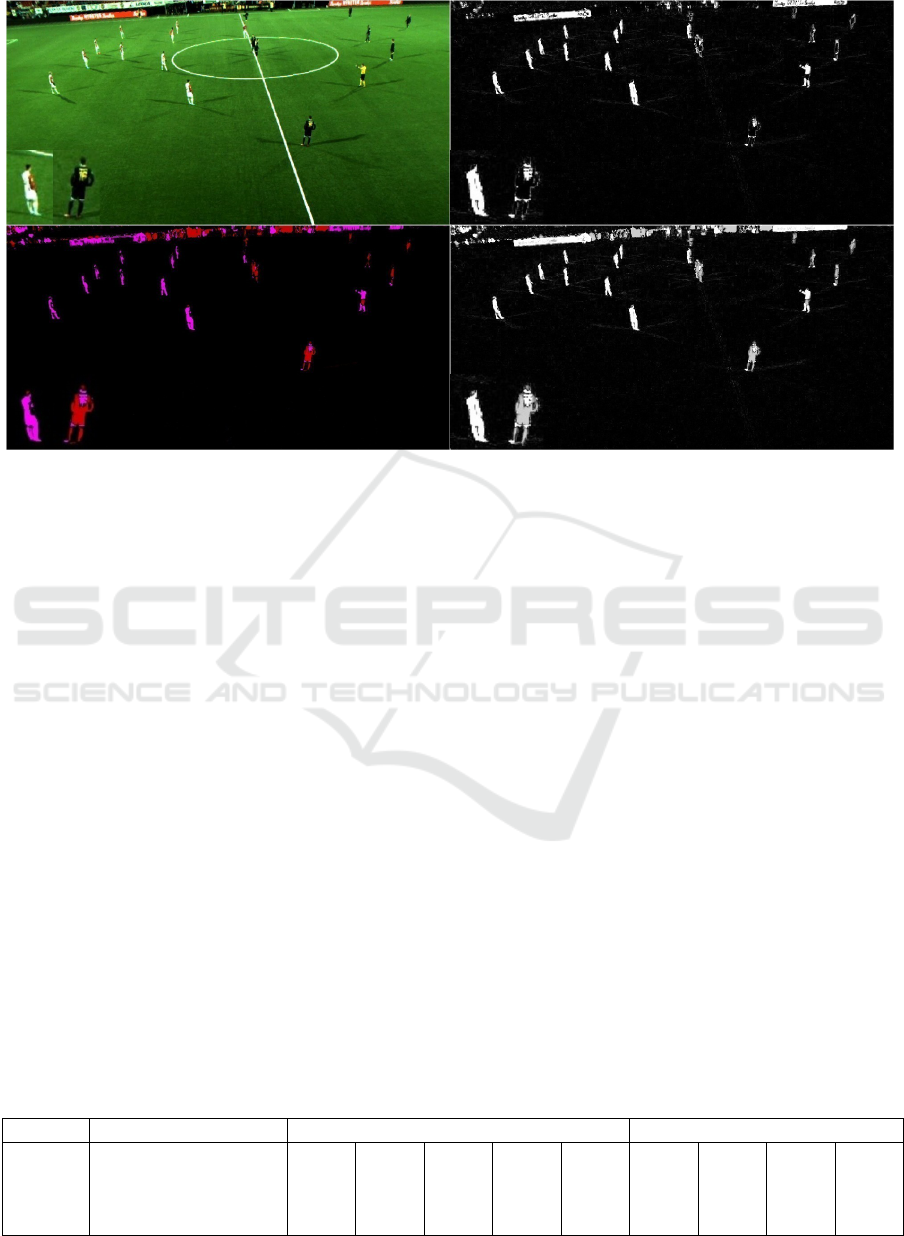
Figure 5: Top-left: Input frame, top-right: foreground objects identified due to high system error, bottom-left: foreground
objects identified due to abnormally low (red) or high(magenta) visibility values, bottom-right: final result. A player from
each team is shown magnified in the bottom-left of each sub-image.
(2) yielding:
I = I
bg
v (4)
The substitution removes the unknown reflectance
term and also the constant illumination term L
?
which
leaves v as the only unknown. Equation (4) holds si-
multaneously for all color channels within the pixel,
with the visibility remaining the same for all three.
This leads to an overdetermined system,
Ax = b (5)
where A is a 3×1 matrix that contains the RGB chan-
nel values of I
bg
, b contains the RGB values of I and
x is the solution to v that we are looking for. We solve
this system using least squares (LS):
x
LS
= (A
T
A)
−1
A
T
b (6)
which can be solved efficiently for a 3 × 1 system.
The relationship between x
LS
, b and the column space
of A is illustrated in Figure 3.
The result of solving Equation (6) for each pixel
within a video frame can be seen in Figure 2 which il-
lustrates that well lit parts have visibility values close
to 1. Furthermore, since we used the background’s
reflectance in our formulation, some of the pixels
that represent the payers whose reflectance does not
match the background, have visibility values outside
the range [0, 1] which are invalid (marked red on Fig-
ure 2).
The error e of the LS solution for the visibility,
defined as
e = kb −Ax
LS
k (7)
is an indication of the overall quality of the least
squares solution (smaller is better). As illustrated in
Figure 3, the error e is the distance of solution v from
the column space of A, hereby denoted as col(A),
which represents the chromaticity of the background.
For a pixel to belong to the background, v must
have valid values and the error e should be small. This
is formalized in the following section which describes
our background model.
Table 1: Configurations tested for each algorithm. The best performing configurations for each algorithm and each dataset
are shown in bold.
Method Metric Football Toscana
MOG2 Mahalanobis distance 64 96 128 160 192 96 128 160 192
GMG Decision threshold .7 .8 .9 .95 .99 .8 .9 .95 .99
ViBe Matching threshold 30 40 50 60 70 15 20 25 30
Ours Decision threshold .1 .2 .3 .4 .5 .01 .05 .1 .15
VISAPP 2017 - International Conference on Computer Vision Theory and Applications
520
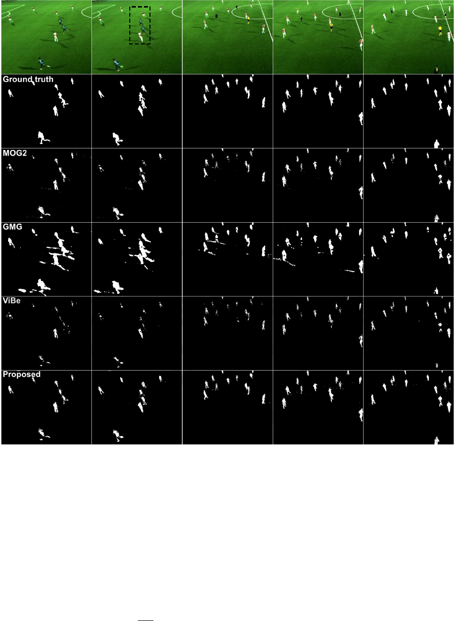
Figure 6: Comparison of MOG2, GMG, ViBe and our method for the football data. A zoomed-in view of the highlighted
region of the second frame can be seen in Figure 7.
2.3 Background Model
Our background model utilizes, at each pixel, the vis-
ibility v obtained using the solution of Equation (6)
and the error e given by (7) in order to estimate the
likelihood for the pixel’s color.
We begin by interpreting e as a measure of dissim-
ilarity between the frame pixel and the background
(e.g. a red-wearing player on a green football field),
Then, the likelihood function:
p(e|BG) = exp
−
e
2
2σ
2
1
(8)
where σ
1
is a model parameter, describes the fact that
background pixels are rarely associated with large
values of e. We have used variance σ
1
= 25 for all ex-
periments, meaning that p(e|BG) significantly drops
when e ≥ 25 units of pixel intensity. A plot of (8)
can be seen in Figure 4a. The top-right image in Fig-
ure 5 shows the result of calculating (8) for each pixel
within a video frame.
It is possible for a foreground object to obtain a
visibility solution with low error e even if it clearly
does not belong to the background. For example, a
player wearing bright green colors on a grass field will
Probabilistic Background Modelling for Sports Video Segmentation
521

Figure 7: Zoomed-in view of the results of the second frame of Figure 6.
have low e since bright green is chromatically close to
grass. To handle such problems, we incorporate the
visibility v in our background model.
Visibility values must, by definition, reside in the
[0, 1] range. It follows that visibility values greater
than 1 are indicative of foreground objects (for exam-
ple players wearing bright colors). Additionally, we
observe that typical sports stadiums are well lit and so
zero illumination areas are unlikely. As a result, very
small visibility values are more likely caused by dark
objects, such as players with dark clothing, rather than
very strong shadows. Based on these observations we
model the likelihood of a pixel’s visibility based on
the background model to be:
p(v|BG) =
exp
−
1
2σ
2
2
(v − v
l
)
2
if v < v
l
1 if v
l
≤ v ≤ v
h
exp
−
1
2σ
2
2
(v − v
h
)
2
otherwise
(9)
where v
l
, v
h
are lower and upper thresholds for the
visibility. Figure 4b illustrates a plot of (9) and Fig-
ure 5 (bottom-left) shows the result of calculating (9)
for each pixel within a video frame. We set v
l
= 0.2,
v
h
= 1 and σ
2
2
= 1.5 for all experiments that follow.
Further to the above, a foreground object may
have a visibility value that is within the allowed range
(v ∈ [v
l
, v
h
]) but have a different color than the back-
ground (e 0). It is also possible for a foreground
object to be chromatically similar to the background
(e ≈ 0) but have abnormal visibility values. Thus,
to model the pixel color’s likelihood given the back-
ground model, equations (8) and (9) are combined to:
p(e, v|BG) = p(e|BG)p(v|BG) (10)
where conditional independence between v and e
stems from the orthogonality between them (see Fig-
ure 3). Figure 4c illustrates the resulting likelihood
function and an application of (10) on each pixel
within a video frame is illustrated in Figure 5 (bottom-
right).
Finally, having obtained the likelihood as per (10),
our algorithm’s final segmentation result is obtained
by thresholding.
3 EVALUATION
For the evaluation of our method we used data from
two football matches (Pettersen et al., 2014) and the
Toscana dataset featuring pedestrians (Maddalena and
Petrosino, 2015). We performed a qualitative and
quantitative comparison against the MOG2 (Zivkovic,
2004) and GMG (Godbehere and Goldberg, 2014)
background segmentation methods as implemented in
OpenCV and the ViBe algorithm (Barnich and Van
Droogenbroeck, 2011) using the implementation pro-
vided by the authors.
We experimented with the decision threshold (or
equivalent) parameter in each algorithm in order to
find a high performing configuration. Additionally,
we investigated other parameters such as the shadow
threshold parameter for the OpenCV implementation
of (Zivkovic, 2004), and found that the default set-
tings produced good results. The images shown in
this paper are those produced by the best-performing
configuration of each algorithm, the parameters of
which are listed in Table 1.
Figure 5 shows a frame from the football video
data and the partial results our method uses to achieve
the the final segmentation. The top-right image shows
foreground objects identified due to high system er-
ror using Equation (8). This metric is able to de-
tect foreground objects that are significantly different,
chromatically, than the background but has problems
with dark objects. The bottom-left image shows fore-
ground objects identified by erroneous visibility val-
ues as given by Equation (9). Red segments indicate
low visibility values and are useful for identifying the
players wearing dark uniforms. The magenta seg-
VISAPP 2017 - International Conference on Computer Vision Theory and Applications
522
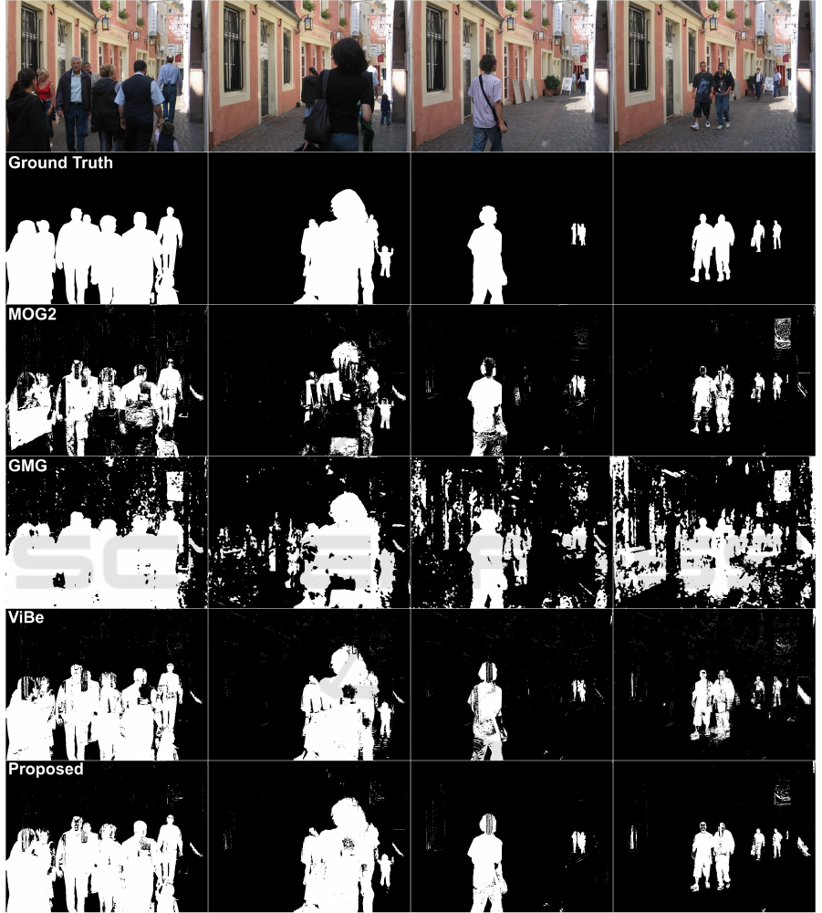
Figure 8: Comparison of MOG2, GMG, ViBe and our method for a scene with pedestrians.
ments indicate visibility values greater than one and
mostly identify the players wearing bright uniforms.
Combining all metrics using Equation (10) gives a
high quality segmentation (bottom-right). It is noted
that the error metric complements the visibility metric
in some cases, such as the red sleeves on the uniforms,
where the visibility happens to be valid (0.2 ≤ v ≤ 1)
but the color does not match the background thus giv-
ing high error values.
Figure 6 compares our method against the MOG2,
GMG and ViBe background subtractors. A ground
truth segmentation is also shown for reference. In
general, our method is able to correctly identify the
players as foreground while also correctly labelling
shadows as background. By contrast other methods
either mislabel shadows as foreground or mislabel
Probabilistic Background Modelling for Sports Video Segmentation
523

1 2 3 4 5 6 7 8 9 10
0.2
0.3
0.4
0.5
0.6
0.7
64
96
128
160
F
1
MOG2
1 2 3 4 5 6 7 8 9 10
0.2
0.3
0.4
0.5
0.6
0.7
64
96
128
160
F
1
MOG2
1 2 3 4 5 6 7 8 9 10
0.2
0.3
0.4
0.5
0.6
0.7
64
96
128
160
F
1
MOG2
1 2 3 4 5 6 7 8 9 10
0.2
0.3
0.4
0.5
0.6
0.7
64
96
128
160
F
1
MOG2
Figure 9: F
1
scores for different configurations of each algorithm for 10 images of the football dataset. The best configuration
is in bold green.
parts of the players as background. This is highlighted
in more detail in Figure 7. MOG2 misidentifies parts
of the player’s pixels (specifically the player on the
top) as background. GMG correctly labels the players
but mislabels parts of shadows as foreground. ViBe
behaves similarly to MOG2 but since it is optimized
for speed instead of accuracy much of the players are
mislabelled. Comparably, our method performs bet-
ter because it captures most of the player silhouettes
while avoiding misidentification of shadows.
Although our method was implemented with the
specific domain of sports in mind, Figure 8 shows
that we obtain good results in more general scenes and
outperform the other methods when dark foreground
objects are present.
Our empirical observations are backed by a quan-
titative evaluation. We manually segmented 5 frames
from each football match (using a 150-frame inter-
val between each frame) and the 6 images from the
Toscana dataset and computed their F
1
scores (Rijs-
bergen, 1979) for various configurations of each algo-
rithm (Table 1). Figure 9 shows the F
1
score for each
configuration running on the football dataset. Our
method consistently outperforms the other methods
for most configurations tested. A similar comparison
was performed to determine the best configuration for
each algorithm for the Toscana dataset (we omit the
graphs due to space constraints). When comparing
the best configuration of each algorithm (Figure 11)
our method outperforms the second-best method by as
much as 10% (5% on average) on the football dataset
and 24% (9% on average) on the Toscana images.
A downside of our model is that it can some-
times misidentify small parts on the players as back-
ground. One such case can be seen in Figure 10.
Because the player is moving quickly, motion blur
blends the color of the player’s leg and the grass turf
behind it producing a dark green color which closely
matches the background when in shadow. As a re-
sult, the algorithm treats that region as shadow and
Figure 10: A failure case. Motion blur causes parts of the
player to match regions in shadow which causes misidenti-
fication.
assigns low foreground probability. Similar problems
appear when applying the MOG2, GMG and ViBe al-
gorithms indicating that a correct decision may not be
possible based on spectral information alone, and that
additional information may be necessary.
4 CONCLUSIONS AND FUTURE
WORK
We have presented a probabilistic background sub-
traction method based on a Lambertian scene model
for the purpose of segmenting sports video data. We
have shown, both through visual comparison and
quantitative measurements, that our method outper-
forms other commonly used background subtraction
methods for two football matches and a more general
scene with pedestrians.
Our algorithm operates on the pixel level making
it amenable to parallelization. In the future, we would
like to optimize and parellelize our implementation
(possibly on the GPU) and compare timings against
other techniques. Some problems remain when deal-
VISAPP 2017 - International Conference on Computer Vision Theory and Applications
524

1 2 3 4 5 6 7 8 9 10
0.2
0.3
0.4
0.5
0.6
0.7
MOG2 GMG
ViBe Ours
F
1
image
1 2 3 4 5 6
0
0.2
0.4
0.6
0.8
1
MOG2 GMG
ViBe Ours
F
1
image
Figure 11: Comparison of the best configuration of each
algorithm for the football and Toscana data. Our algorithm
consistently outperforms the other methods for the football
dataset and is better for most images of the Toscana dataset.
ing with fast-moving objects that blend with the back-
ground. We plan to explore solutions to these prob-
lems using texture and geometric information. An-
other direction would be to experiment with color
spaces other than RGB whose channels are less cor-
related as it could increase the quality of our least
squares solution. Lastly, we plan to extend the pro-
posed method to operate under variable illumina-
tion conditions, dynamic backgrounds, and non-static
cameras.
REFERENCES
Barnich, O. and Van Droogenbroeck, M. (2011). ViBe:
A Universal Background Subtraction Algorithm for
Video Sequences. IEEE Transactions on Image Pro-
cessing, 20(6):1709–1724.
Chen, C.-C. and Aggarwal, J. (2010). Human Shadow Re-
moval with Unknown Light Source. In 20th Interna-
tional Conference on Pattern Recognition, volume 27,
pages 2407–2410, Istanbul, Turkey.
Duncan, K. and Sarkar, S. (2012). Saliency in images and
video: a brief survey. IET Computer Vision, 6(6):514–
523.
Godbehere, A. B. and Goldberg, K. (2014). Algorithms for
Visual Tracking of Visitors Under Variable-Lighting
Conditions for a Responsive Audio Art Installation.
In Controls and Art, pages 181–204. Springer Inter-
national Publishing, Cham.
Graham, T. (2012). Sports tv applications of computer
vision. BBC Research & Development White Paper
WHP220.
Hsieh, J.-W., Hu, W.-F., Chang, C.-J., and Chen, Y.-
S. (2003). Shadow elimination for effective moving
object detection by Gaussian shadow modeling. Im-
age and Vision Computing, 21(6):505–516.
Huerta, I., Amato, A., Roca, X., and Gonz
´
alez, J. (2013).
Exploiting multiple cues in motion segmentation
based on background subtraction. Neurocomputing,
100:183–196.
Kaimakis, P. and Tsapatsoulis, N. (2013). Background
Modeling Methods for Visual Detection of Maritime
Targets. In In Proc. Int. Workshop on Analysis and
Retrieval of Tracked Events and Motion in Imagery
Stream, pages 67–76, Barcelona, Spain.
Khan, S. H., Bennamoun, M., Sohel, F., and Togneri,
R. (2014). Automatic Feature Learning for Robust
Shadow Detection. In Proc. Conf. Comp. Vision and
Pattern Recognition, pages 1939–1946, Columbus,
Ohio, USA.
Leone, A. and Distante, C. (2007). Shadow detection for
moving objects based on texture analysis. Pattern
Recognition, 40(4):1222–1233.
Levin, A., Lischinski, D., and Weiss, Y. (2008). A Closed-
Form Solution to Natural Image Matting. Trans. Pat-
tern Analysis and Machine Intelligence, 30(2):228–
242.
Maddalena, L. and Petrosino, A. (2015). Towards Bench-
marking Scene Background Initialization. In Proc
Int. Conf. Image Analysis and Processing, volume
9281, pages 469–476.
Perazzi, F., Krahenbuhl, P., Pritch, Y., and Hornung,
A. (2012). Saliency filters: Contrast based filtering
for salient region detection. In Proc. Conf. Comp. Vi-
sion and Pattern Recognition, pages 733–740.
Pettersen, S. A., Halvorsen, P., Johansen, D., Johansen,
H., Berg-Johansen, V., Gaddam, V. R., Mortensen,
A., Langseth, R., Griwodz, C., and Stensland, H. K.
(2014). Soccer video and player position dataset. In
Proc. Multimedia Systems Conf., pages 18–23, New
York, USA.
Rijsbergen, C. J. V. (1979). Information Retrieval.
Butterworth-Heinemann, Newton, MA, USA, 2nd
edition.
Sanin, A., Sanderson, C., and Lovell, B. C. (2010). Im-
proved Shadow Removal for Robust Person Tracking
in Surveillance Scenarios. In Proc. Int. Conf. on Pat-
tern Recognition, pages 141–144.
Sanin, A., Sanderson, C., and Lovell, B. C. (2012). Shadow
detection: A survey and comparative evaluation of re-
cent methods. Pattern Recognition, 45(4):1684–1695.
Shahrian, E., Rajan, D., Price, B., and Cohen, S. (2013). Im-
proving Image Matting Using Comprehensive Sam-
pling Sets. In Proc. Conf. Computer Vision and Pat-
tern Recognition, pages 636–643.
Stone, J. E., Gohara, D., and Shi, G. (2010). OpenCL:
A Parallel Programming Standard for Heterogeneous
Computing Systems. Computing in Science & Engi-
neering, 12(3):66–73.
Wang, J. and Cohen, M. F. (2007). Image and Video Mat-
ting: A Survey. Foundations and Trends in Computer
Graphics and Vision, 3(2):97–175.
Yan, Q., Xu, L., Shi, J., and Jia, J. (2013). Hierarchical
saliency detection. In Proceedings of the IEEE Con-
ference on Computer Vision and Pattern Recognition,
pages 1155–1162.
Zivkovic, Z. (2004). Improved adaptive Gaussian mixture
model for background subtraction. In Proc. 17th In-
ternational Conf. on Pattern Recognition, volume 2,
pages 28–31 Vol.2, Washington, DC, USA.
Probabilistic Background Modelling for Sports Video Segmentation
525
