Generative Animation in a Physics Engine using Motion Captures

Brian Wilke and Sudhanshu K. Semwal

Department of Computer Science, University of Colorado, Colorado Springs, CO, 80918, U.S.A.

Keywords:

Articulated Motion, Motion Capture, Novel Application, Asymmetric Scaling, Under Controlling.

Abstract:

Motion captures are an industry standard for producing high-quality, realistic animations. However, generat-

ing novel animations from motion captures remains a complex, non-trivial problem. Many techniques have

been developed, including kinematics and manually solving the equations of motion. We present a new tech-

nique using a physics engine to generate novel animations. Motion captures are effectively simulated within

a popular open-source physics engine, Bullet, and two generative techniques are applied. These generative

techniques – asymmetric scaling and under-controlling – are shown to be simple and straight-forward. The

techniques and methods were implemented in Python and C++, and show new promising avenues for genera-

tive animation using existing motion captures.

1 INTRODUCTION

Motion capture has become an industry standard for

producing high-quality, realistic animations in ﬁlm

and games (Schreiner and Gleicher, 2002; Calvert

et al., 2002; Multon, 1999; Boulic et al., 1990; Hod-

gins, 1996; Macchietto et al., 2009; Ryan, 1990), and

pivotal papers describing a general purpose rigid body

collision and contact simulator (Baraff, 1989; Baraff,

1991). However, once motion capture data is sam-

pled, it is difﬁcult to adjust and re-target. A common

example of this distortion is footskate, where the char-

acter’s feet move when they really should be planted

(Schreiner and Gleicher, 2002). Furthermore, what if

the director wants the right arm above the head in-

stead of on the waist, and the left leg bent instead of

straight? A new motion capture must almost certainly

be taken, since adjusting the original capture would

be too time-consuming, expensive, and possibly un-

realistic.

1.1 Generating Novel Animations with

Motion Captures

Adjusting motion captures has been a continuing ﬁeld

of study, especially since captures have inherent ob-

stacles to overcome, e.g., footskate. A main ques-

tion has been whether a capture or set of captures can

be used to generate novel animations. For instance,

given a particular walking capture, can we adapt it to

a different skeleton walking at a different speed?

This particular type of generative animation is

called walking motion synthesis. There have been

three main previous research directions in this area,

presented in (Multon, 1999): kinematics, solving the

equations of motion, and interpolation.

Kinematics is the geometry of motion. This ap-

proach speciﬁes key joint angles that determine the

rest of the model’s conﬁguration. This method can

generate various synthesizers, as in (Boulic et al.,

1990). However, as in all kinematics, it can require

massaging from the animator to provide physical re-

alism and avoid mechanical movements.

Solving the equations of motion attempts to ﬁnd

the correct forces and torques to apply to reach a cer-

tain position. (Hodgins, 1996) models humans run-

ning physically and directly computes the forces and

torques required for running (Hodgins, 1996). Con-

trollers have to be implemented to avoid impossible

joint conﬁgurations. In (Macchietto et al., 2009), a

real-time simulation system automatically balances

a standing character, deriving the mechanics of bal-

ance from linear and angular momentum. Interpo-

lation edits motion capture data between given mo-

tions. (Ashraf and Wong, 2000) interpolate walking

and running motions and generate a new motion be-

tween four given motions (Ashraf and Wong, 2000).

(Rose et al., 1998) use multivariate interpolation on

classiﬁed motion, generating a new animation by ap-

plying polynomial and radial basis function interpo-

lation between B-Spline coefﬁcients under the classi-

ﬁcation (Rose et al., 1998). Extrapolation is not pos-

250

Wilke B. and Semwal S.

Generative Animation in a Physics Engine using Motion Captures.

DOI: 10.5220/0006134702500257

In Proceedings of the 12th International Joint Conference on Computer Vision, Imaging and Computer Graphics Theory and Applications (VISIGRAPP 2017), pages 250-257

ISBN: 978-989-758-224-0

sible with these techniques, and the parameters can

be quite difﬁcult to properly set. PCA has also been

introduced into animation synthesis. (Glardon et al.,

2004) use principal component analysis (PCA) to cre-

ate a walking engine based on motion captures (Glar-

don et al., 2004). This engine computes the walking

cycle for different skeleton sizes at different speeds.

Controlling Independent Rigid Bodies. Let the

rigid body for joint j be r

( j). At each frame

f , a joint’s rigid body r

( j) has a linear velocity

v(r

( j), f ) computed by the physics engine. This ve-

locity is computed given the forces acting on r

( j),

e.g., gravity. Our target linear velocity from the mo-

tion capture for joint j in the next frame f + 1 is

v( j, f + 1). The error term between our current and

target velocities is then

( j, f ) = v( j, f + 1) − v(r

( j), f ), (1)

where j is the joint, f is the frame, v( j, f + 1) is

our calculated linear velocity in the next frame, and

v(r

( j), f ) is the physics engine’s computed linear ve-

locity on the rigid body r

( j) in f . This error term

allows us to control the rigid body r

( j)’s linear ve-

locity in the presence of other forces.

A proportional control loops uses only a propor-

tional term for the next output, that is, P

out

= K

e(t),

where P

out

is the loop’s output at time t, e(t) is the sys-

tem’s error at t, and K

is the proportionality constant.

Using this kind of control loop, between frames f and

f + 1, we apply a central force to each rigid body

F( j, f ) = K

· m(r

( j)) · e

( j, f ), (2)

where j is the joint, r

( j) is the rigid body corre-

sponding to j, m(r

( j)) is r

( j)’s mass > 0, K

an appropriately chosen constant, and e

( j, f ) is from

Equation (1). This equation incorporates all forces

acting on the body and applies a force that will cor-

rect its motion to our target motion from the motion

capture.

Having developed simple controllers for indepen-

dent rigid bodies, we can consider the problem of cre-

ating a physical skeleton. The motion capture joint

hierarchy speciﬁes the parents and children of each

joint. Typically, it is a rooted tree where each joint

has one unique parent. We will assume that is the

case, such that H : J → G where G is a tree and ∃ j ∈ J

such that j is the root of G.

Asymmetric Scaling and Under-controlling. Now

that we have a physics engine that replicates the orig-

inal motion capture’s motion, we can consider gener-

ating novel animations using this data. Here, we will

consider two types of generative animation: asym-

metric scaling and under-controlling. These tech-

niques can exist on their own or combine together to

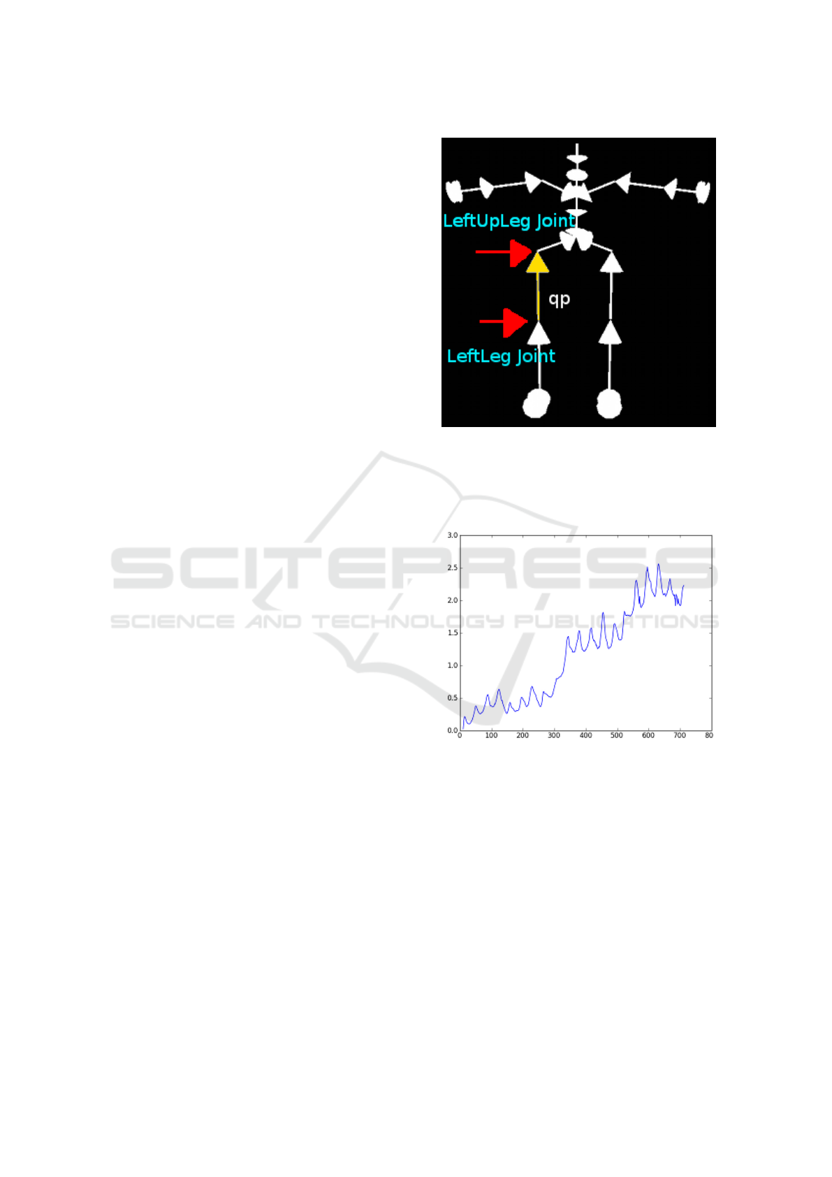
Figure 1: The various q

( j) vectors between joints and par-

ent joints in a motion capture hierarchy H. The LeftUpLeg

joint and LeftLeg joint are marked in the picture, and the

(LeftLeg) vector between them is highlighted. In this

particular hierarchy, the LeftUpLeg joint is a parent of the

LeftLeg joint.

Figure 2: This graph plots e

( j, f ) for j = Hips against the

frame numbers. Though there is some oscillation, the er-

rors appear to accumulate over time, causing a left-to-right

upwards slope in the graph.

generate new animations. Asymmetric scaling sim-

ulates what would happen to the original motion if,

e.g., part of the body became stronger. For instance,

consider a motion capture of a boxer shadow box-

ing. The boxer wants to increase the power of his

punches. With asymmetric scaling, we can simulate

what would happen to his shadow boxing if he in-

creased his biceps muscle mass, or his shoulder mus-

cle mass, or his abdominal muscle mass, etc. By in-

cluding a proportional term,

( j, f ) = K

( j, f ) · v( j, f ), (3)

Generative Animation in a Physics Engine using Motion Captures

251

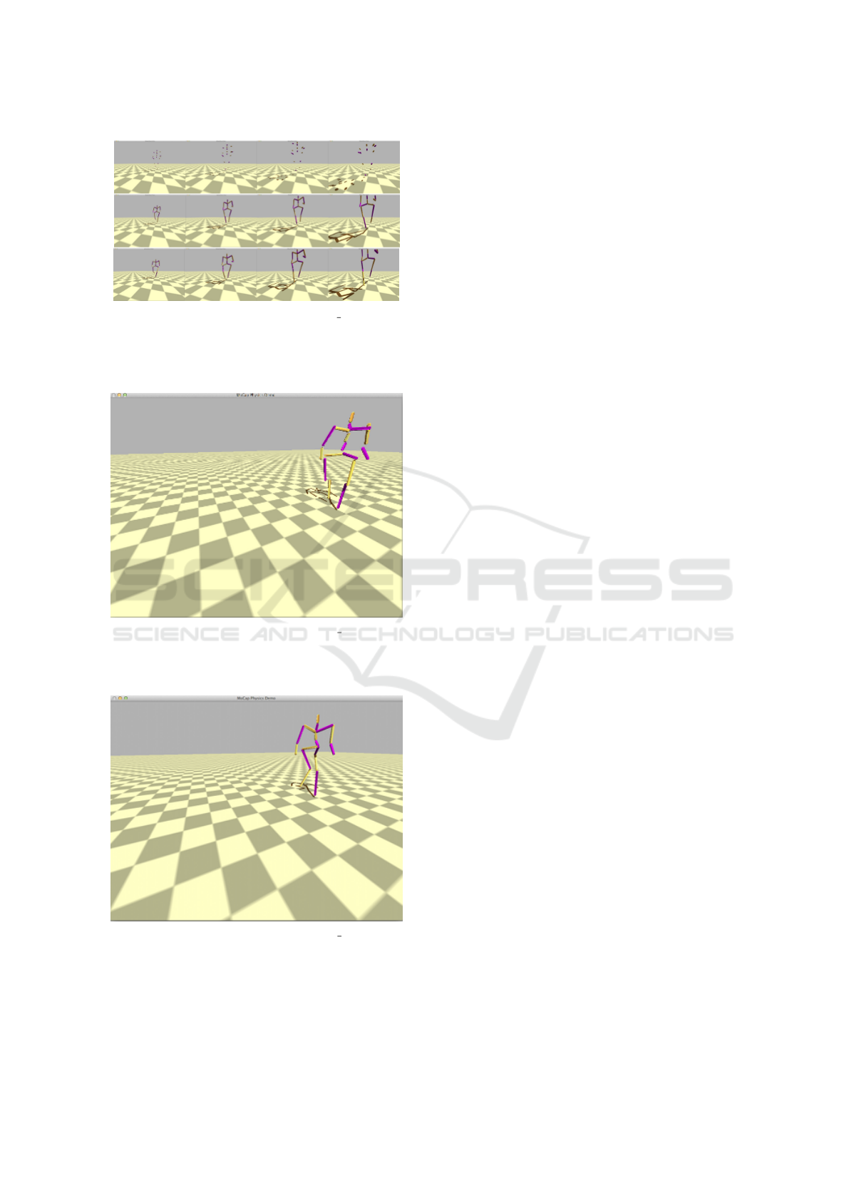
Figure 3: Simulated animation stills of 141 02.bvh using

independent rigid bodies, a physical skeleton, and a con-

strained physical skeleton, respectively from top to bottom,

using the tuned parameters.

Figure 4: A still from the simulation of 141 30.bvh using

physical skeletons after many steps. The error has accu-

mulated enough that joints that should remain locked are

drifting away from each other.

Figure 5: A still from the simulation of 141 30.bvh using

constrained physical skeletons after many steps. The ani-

mation looks much better because the joints remain locked

together.

we simulate a change in joint velocity, where v( j, f )

is joint j’s linear velocity in frame f . This velocity

scaling also simulates what would happen if, e.g., a

tennis player swung her racket harder or softer, or a

cyclist pedalled harder or softer during a climb. That

is, this approach can simulate a velocity change that is

within a person’s reach given their current physicality.

A tennis player could utilize this technique to deter-

mine optimal swinging speed for a given ball, where

the velocity change transferred to the racket changes

the trajectory of the ball. The ball’s trajectory change

could also be physically simulated in our physics en-

gine.

1.2 Under-controlling

In our previous techniques, we exactly speciﬁed a

controller on every rigid body in the physical skele-

ton. With a physical skeleton operating under con-

straints, this exact speciﬁcation is not required. Rigid

body constraints determine how two rigid bodies can

transform with respect to each other. As mentioned

earlier, the shoulder is a type of ball and socket joint

that limits translation away or towards the humerus

and the shoulder blade, but allows rotation. This ball

and socket constraint is also known as a point-to-point

constraint. In general, 3d macroscopic rigid bodies

have 6 degrees of freedom (DoF): translation along

any axis, and rotation about any axis. A point-to-

point constraint is a specialization where the transla-

tions are locked, i.e., there are only the 3 rotational de-

grees of freedom. A generic 6 DoF constraint can be

created which limits or does not limit any particular

DoF. Applying these constraints to each pair of rigid

bodies in our physical skeleton allows us to under-

control the skeleton. The physics engine will update

each rigid body’s position based on our control loop

and the rigid body’s constraints. For instance, we

could control only the right side of the body, which

would create a zombie-like effect where the left side is

limply carried along. Our joints – the location where

bones connect – have very well-deﬁned constraints.

In fact, dislocations occur when we violate these con-

straints. We have already touched upon the shoulder’s

constraint, but other major constraints include the el-

bow, the wrist, and the knee. For instance, as part

of the elbow, the radius and ulna (the bones of the

forearm) can rotate around the two axes perpendicu-

lar to the elbow, but not by more than the proximal

semicircle deﬁned by the axis of the humerus, and the

humerus, radius, and ulna cannot translate with re-

spect to each other. Most joints in the human body do

not allow translations, but allow rotations. By spec-

ifying these constraints, we can free ourselves from

controlling every rigid body.

GRAPP 2017 - International Conference on Computer Graphics Theory and Applications

252

2 ALGORITHM DEVELOPMENT

AND IMPLEMENTATION

The code developed for this paper uses a mix of

Python and C++, and utilizes the Bullet physics en-

gine (Coumans, 2012). Only the BVH motion capture

ﬁle format is supported, though other formats such as

ASF/AMC could be added in the future as necessary.

The intent is to work with the large CMU Graphics

Lab Motion Capture Database and compare the orig-

inal motion captures to the generated physics anima-

tion (Calvert et al., 2003; Club, 2013). Even though

the CMU Database uses the ASF/AMC format origi-

nally, their captures have been exported to the BVH

format, and BVH is more compatible with certain

tools that sped development, such as ply, an imple-

mentation of lex and yacc in Python (Beazley, 2011;

OpenGL, 2013; SciPy, 2013; Evans, 2011). There is

no appreciable difference between the BVH ﬁles we

use here and the original ASF/AMC ﬁles, except for

the ﬁrst frame which includes a T-pose of the cap-

ture’s hierarchy.

Five motion captures from the CMU motion cap-

ture database were replicated physically and had gen-

erative techniques applied.

Replicating the Motion Physically and Positional

Error. Our controllers depend on two variables: the

numerical differentiation technique and the propor-

tionality constant. We evaluated central differences

with various orders, ∇(n), where n is the order and

1 ≡ n mod 2. With each order, we also tuned the pro-

portionality constant K

to minimize positional error

across all joints. Because we also scale our model in

our simulation, there is a second tuning constant, K

which scales our velocities symmetrically. That is,

( j, f ) = K

v( j, f ),

for all joints j in all frames f , where v( j, f ) is joint

j’s linear velocity in frame f .

Our goal is to search for a central difference ∇(n)

and a pair (K

) that minimizes differences be-

tween the original motion capture and the simulation.

For a joint j in frame f , its positional error vector is

( j, f ) = r( j, f ) − ρ

ρ(r

( j), f ),

where ρ

ρ(r

( j), f ) is the position of the rigid body

( j) that corresponds to joint j in frame f , and

r( j, f ) is j’s position in the motion capture in frame

f . In an independent rigid body, ρ

ρ is the rigid body’s

center of mass, whereas for a physical skeleton, it is

at one end of the capsule shape we use for r

( j). The

squared error is

( j, f ) = e

( j, f ) · e

( j, f ),

which is just the dot product of e

with itself. Aver-

aging across all frames, we get

¯e

( j) =

| f |

∑

( j, f ),

where | f | is the number of frames. Finally, averaging

across all joints, we achieve an error number for each

pair (K

) and central difference ∇(n)

¯e

,∇(n)) =

|J|

∑

j∈J

¯e

( j). (4)

Minimizing Equation (4) gives us tuned parame-

ters that closely match the simulation to the original

motion capture.

Search Algorithm. There are many algorithms we

could use to search for the parameters (K

,∇(n))

that minimize Equation (4). One rather simplistic ap-

proach is to generate random triples of numbers, cal-

culate Equation (4) for each triple, and compare. This

kind of search is known as a Monte Carlo search, and

is very applicable when the domain of the triples is

limited and it is difﬁcult to obtain or apply a deter-

ministic method that optimizes these parameters. In-

deed, formulating a deterministic method appears ex-

tremely difﬁcult, since, not only do we apply forces

and torques to each rigid body, but Bullet too applies

the force of gravity and constraint forces to each rigid

body in each frame. We therefore used a modiﬁed

Monte Carlo search. We limited our central differ-

ences to orders 3 ≤ n ≤ 19. For certain (K

the rigid bodies can literally ﬂy apart in the simu-

lation, so we seed the search initially with a known

good pair, (K

). Algorithm 1 details the search

method, where random[−1, 1] is a function that pro-

duces a random real number, i.e., a ﬂoating point

number, between -1 and 1 inclusive. It can easily be

seen that this algorithm runs in O(points · maxOrder ·

F(mocap-ﬁle)), where F is the number of frames in

mocap-ﬁle.

We found that a good starting point for indepen-

dent rigid bodies was (K

) = (100, 75), and for

physical skeletons was (K

) = (20,100). These

parameters produced a simulation that at least some-

what matched all of the captures. We then tuned to

a single motion capture, 141 15.bvh. This capture is

by far the longest of our 5, and demonstrates many

interactions between joints by going through ranges

of motion. From there, we used 100 points per run,

each run taking about 14 minutes on a laptop, and a

maximum order of 19. We then used the best tun-

ing parameters from each run to seed the good values

of the subsequent run. A concern with this particular

method is that runs will not converge upon a better

solution. However, we found that, starting with the

Generative Animation in a Physics Engine using Motion Captures

253

Table 1: Tuned parameters for independent rigid bodies and physical skeletons.

Rigid Body n K

¯e

points Runs

Independent Rigid

Bodies

5 98.5331 85.46 0.511 0.561 100 5

Physical Skeleton 5 32.5875 86.419 0.874 0.660 100 9

Constrained Physical

Skeleton

3 24.1933 120.798 1.472 0.999 100 10

Algorithm 1: Tuning parameters with a Monte Carlo search.

function TUNE-PARAMETERS(K

, points,

maxOrder, mocap-ﬁle)

← K

∇ ← {}

for i = 3 → maxOrder,1 ≡ i mod 2 do

∇ ← {central-difference(i,r)}

end for

f ,b

← K

vc,b

← K

,∇

← ∇(3)

¯e

← ∞

for i = 1 → points do

for ∇(n) ∈ ∇ do

¯es

= run simulation of mocap-ﬁle with

)

if ¯es

< ¯e

then

¯e

= ¯es

f ,b

← K

vc,b

← K

,∇

← ∇(n)

end if

← K

+random[−1,1]

← K

c+random[−1,1]

end for

return ¯e

f ,b

vc,b

,∇

end function

good points, we achieved convergent results with

a small number of runs. The tuning results for

141 15.bvh are listed in Table 1. These results show

that we can minimize the error between our simula-

tion and a motion capture simply and effectively. To

speed calculations of averages, and avoid errors such

as massive cancellation, we used an algorithm due to

Knuth and Welford (Knuth, 1998). This algorithm

can calculate an average and standard deviation in one

pass of the data. We use it during our simulation. In

Algorithm 2, we present our use of the method for the

positional errors of each joint. The same algorithm is

used to aggregate the joint positional errors into our

overall average error.

As with any controller, the parameters in Table

1 may work great for a speciﬁc instance, but break-

down for another. These results are repeatable, simu-

lation after simulation. Longer captures accumulated

greater error, as shown in Figure 2.

Algorithm 2: Online average calculation.

∀ j ∈ J, ¯e

( j) ← 0, n( j) ← 0,M

( j) ← 0

for j ∈ J at each step s, f of the simulation do

n( j) ← n( j) + 1

∆ ← e

( j, f )− ¯e

( j)

¯e

( j) ← ¯e

j +

∆

n( j)

( j) ← ∆( ¯e

( j, f )− ¯e

( j)

end for

( j) = M

( j)/(n( j) − 1)

Animations using the Tuned Parameters. In Fig-

ure 3, we present animation stills from within a single

simulation. Each type of rigid bodies was simulated

on a single ﬁle, 141 02.bvh. The camera remained

at the same place as the independent rigid bodies, the

physical skeleton, and the constrained physical skele-

ton were simulated in turn.

Figure 4 shows the physical skeleton after it has

turned around and is walking back towards its orig-

inal position in the simulation of motion capture ﬁle

141 30.bvh. Figure 5 shows the constrained physical

skeleton at the same point in 141 30.bvh. The dis-

connections in Figure 4 are gone from 5 because of

the Bullet constraints placed on the joints. Coupled

with the tuned parameters, constraints offer a pow-

erful animation enhancement. To demonstrate our

two generative animation techniques, we used our ﬁve

motion capture ﬁles. For instance, 141 14.bvh cap-

tures punching and kicking, which is a good candi-

date to show how scaling, e.g., the left foot, changes

the kicks, and 141 30.bvh captures a random walk,

which is a good candidate for showing how under-

controlling can produce, e.g., a zombie-like anima-

tion. All of our generative animations used a con-

strained physical skeleton.

2.1 Asymmetric Scaling

By scaling K

( j, f ), we found that we could make the

kicks of 141 14.bvh harder or softer easily. For in-

stance, by scaling the right foot by

(RightFoot,200 ≤ f ≤ 600) = 1.2,

we simulated a harder snap between the right knee

and foot, as compared in Figure 6.

GRAPP 2017 - International Conference on Computer Graphics Theory and Applications

254

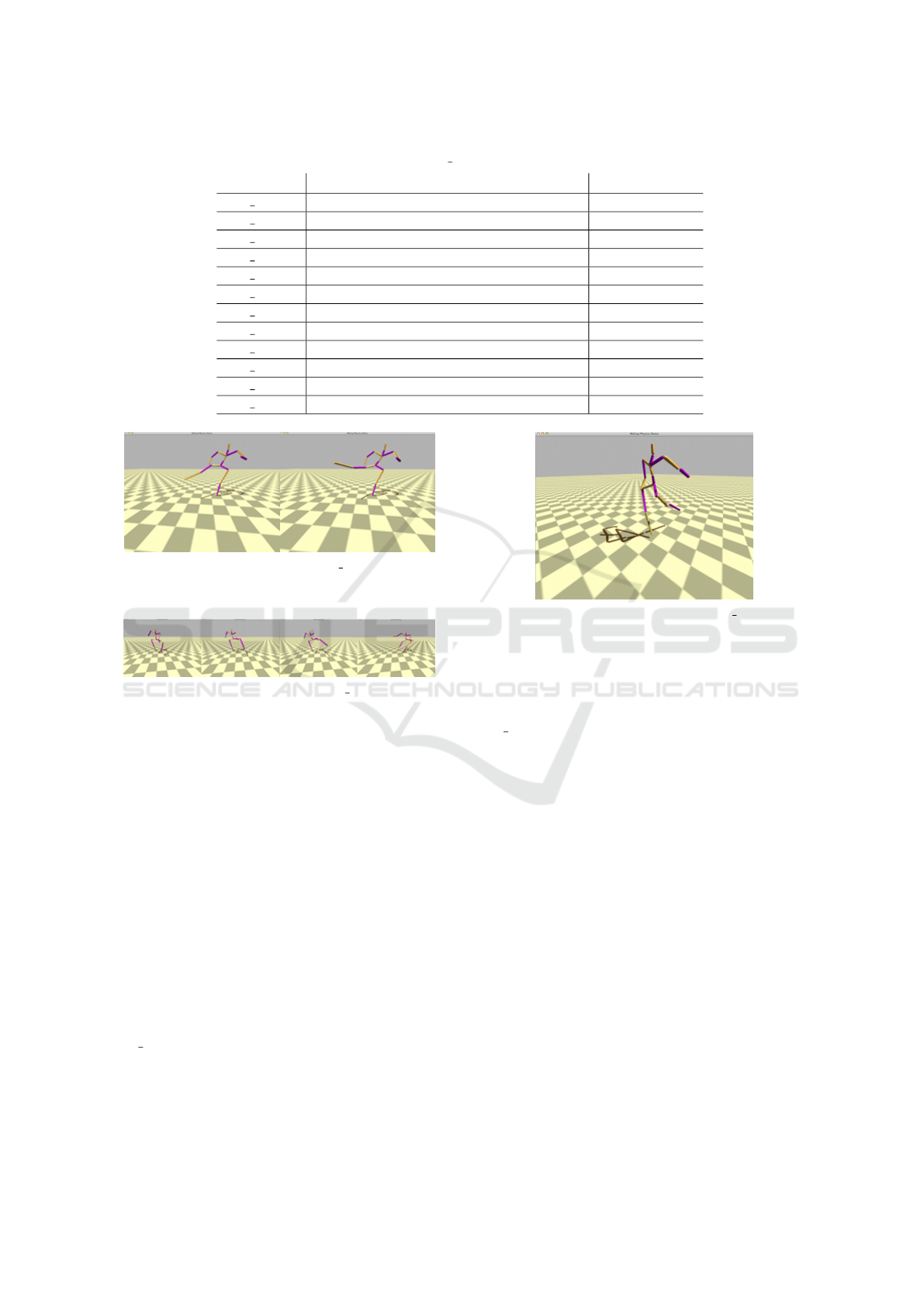
Table 2: Comparison of errors using 141 15.bvh tuned parameters with other captures.

File Rigid Body ¯e

141 02.bvh Independent Rigid Bodies 3.431 0.194

141 02.bvh Physical Skeleton 3.262 0.174

141 02.bvh Constrained Physical Skeleton 0.669 0.022

141 08.bvh Independent Rigid Bodies 2.992 0.023

141 08.bvh Physical Skeleton 2.389 0.020

141 08.bvh Constrained Physical Skeleton 0.237 0.007

141 14.bvh Independent Rigid Bodies 0.121 0.0005

141 14.bvh Physical Skeleton 0.234 0.012

141 14.bvh Constrained Physical Skeleton 0.395 0.042

141 30.bvh Independent Rigid Bodies 4.612 0.029

141 30.bvh Physical Skeleton 3.220 0.071

141 30.bvh Constrained Physical Skeleton 0.893 0.164

Figure 6: Stills from simulations of 141 14.bvh comparing

the original, un-scaled simulation on the left to a simulation

using asymmetrical scaling on the RightFoot on the right.

Figure 7: Stills from simulations of 141 15.bvh using the

asymmetrical scaling from Table 4.

In the original simulation, at the height of the kick,

the right leg stays below ground-parallel, the left leg

is bent, the left hip is more ground-parallel, the left

elbow is bent into the body, and the spine is bent only

slightly towards the left side of the body. In the scaled

simulation, at the height of the kick, the right leg is

ground-parallel or more, with the knee actually bent

past 90 degrees, the left leg is less bent, the left hip is

less ground-parallel, the left elbow is bent more away

from the body, and the spine is bent more towards the

left side of the body. Just by applying an asymmet-

ric scale to the RightFoot, we substantially changed

the resultant forces and torques on the entire leg, the

Spine, the LeftHand, even the Head! If a kickboxer

kicks 1.2 times harder with his feet, this simulation

shows what happens to his entire body.

We also applied asymmetric scaling on

141

15.bvh using multiple different scales dur-

ing the entire simulation. The different scales are

listed in Table 4. The resulting animation shows what

would happen if the left side of the body became

signiﬁcantly stronger than the right side, and is quite

Figure 8: A still from the simulation of 141 30.bvh using

an under-controlled constrained physical skeleton where the

left hand and left foot are not controlled. The hand and foot

lift up because of their constraints with their parent bodies

and joints.

comical. Figure 7 shows stills from a simulation of

141 15.bvh using the scales in Table 4 where the left

arm actually goes under the left leg.

While comical, this generation also demonstrates

how someone recovering from a serious injury will

be impacted. For instance, a person who does injure

their right leg severely and must keep off of it will ex-

perience decreased muscle mass in the right leg, and

potentially increased muscle mass in their left leg to

compensate. This imbalance will lead to very unex-

pected results as the person begins using their right

leg again, as demonstrated here.

2.2 Under-controlling: Zombies

Furthermore, a gimp leg does not rotate at the knee.

So, instead of a point to point constraint, we used

a generic 6 DoF constraint locked in all axes at the

knee and hand. We also changed the mass of the three

bodies in the chain between the foot and the hip and

the hand and the shoulder. We found that the foot

mass should be lower than the leg mass, and the hand

mass should be lower than the arm mass, to produce

Generative Animation in a Physics Engine using Motion Captures

255

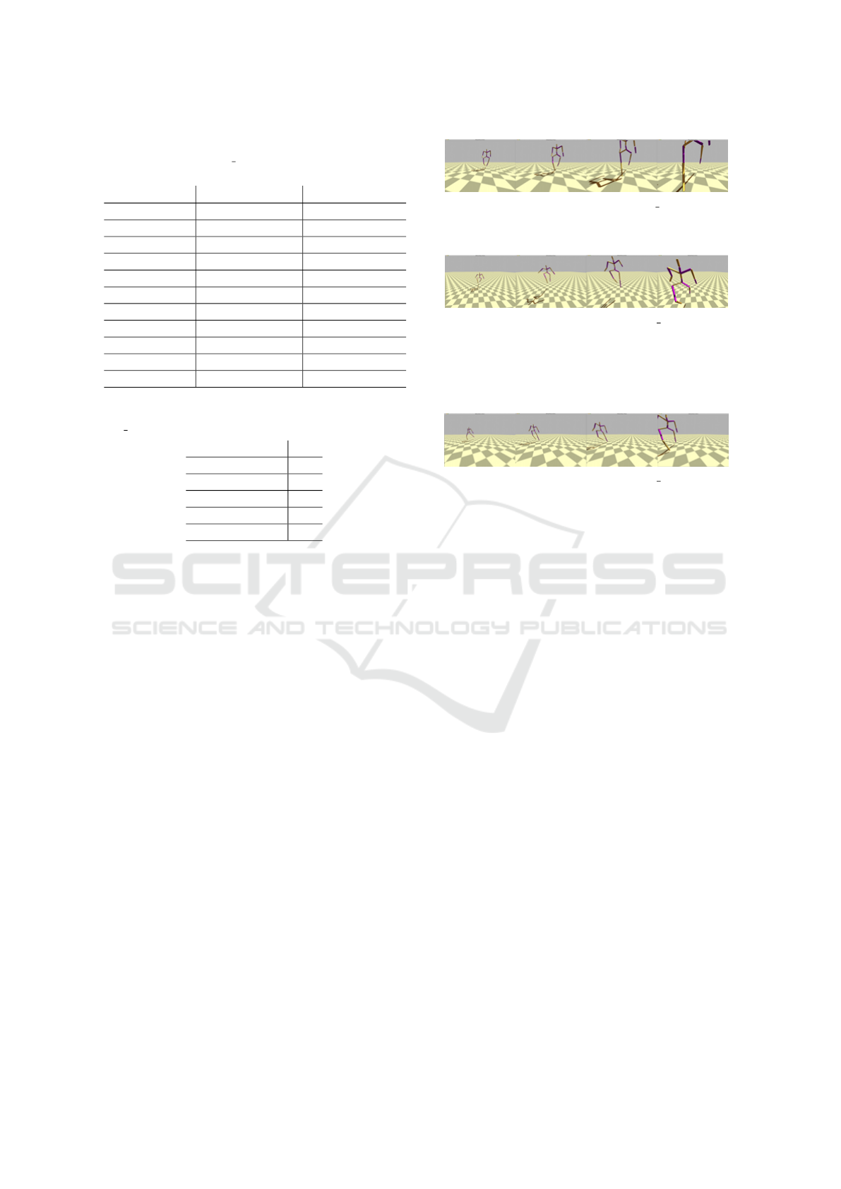
Table 3: Comparison of the forces on certain joints of an

un-scaled and scaled 141 14.bvh simulation. The scaling is

solely applied to the RightFoot.

Joint j

( j),r

( j))

( j),r

( j))

RightFoot 15.196 23.643

RightLeg 4.458 1.640

RightUpLeg 1.618 2.548

Spine 0.148 0.554

LeftFoot 0.0987 0.0949

LeftLeg 0.084 0.143

LeftUpLeg 0.307 1.043

LeftHand 0.009 0.145

LeftForeArm 0.002 0.002

LeftArm 0.008 0.002

Head 0.010 0.008

Table 4: The asymmetric scales used to simulate

141 15.bvh. Values for joints are given.

Joint j K

LeftFoot 1.1

RightFoot 0.9

LeftHand 1.5

RightHand 0.5

All other joints 1.0

the desired animation. These bodies are less massive

on the human body, and, zombies being anatomically

human, this result is most expected. Masses for Left-

Foot, LeftLeg, LHipJoint, LeftHand, LeftFOreArm,

and LeftArm are: 5, 10, 20. .25, 2.0, and 5 respec-

tively. All other joints are 1 units.

3 CONCLUSIONS AND FUTURE

WORK

Using Python, C++, and the Bullet Physics library, a

motion capture to linear velocity transformer was im-

plemented. This transformer relied on two techniques

with three parameters: numerical differentiation us-

ing central differences with one parameter, the order,

and proportional controllers with two parameters, the

actual proportionality constant for the controller and

a symmetric scaling constant. We also showed how,

using this transformer, we could achieve two gener-

ative animation techniques: asymmetric scaling and

under-controlling. The results showed that replicat-

ing the original motion capture in a physics engine

is feasible, though the proportional controllers tend

to accumulate errors over time. Tuning the param-

eters to a single capture was fairly simple using a

Monte Carlo method, and these parameters worked

well across other captures. Physical skeletons tended

Figure 9: Stills from a simulation of 141 02.bvh using a

zombie physical skeleton. We can see that the left leg’s knee

does not bend at all.

Figure 10: Stills from a simulation of 141 08.bvh using a

zombie physical skeleton. The motion capture actor steps

up onto a platform and then down. The platform is not

shown here. We can see that the skeleton looks awkward

stepping down from its left leg onto its right, since the left

leg is locked and does not bend at the knee.

Figure 11: Stills from a simulation of 141 30.bvh using a

zombie physical skeleton. We can see that the left side of

the body is limp corresponding to a shufﬂing zombie.

to produce defects at the parent joint of a rigid body

over time. Constrained physical skeletons compen-

sated for these defects and created good-looking an-

imations. We found that generating new animations

in the physics simulations achieved intriguing results.

Asymmetrical scaling can be achieved simply; chang-

ing only one joint slightly in a few frames caused no-

ticeable and interesting changes in the simulation. We

also showed how under-controlling could achieve a

zombie-like effect by under-controlling certain rigid

bodies on the left-side of a constrained physical skele-

ton. By recreating motion captures in a physics en-

gine, we hoped to overcome previous dynamics gen-

eration limitations. Possible uses of this work include

sports medicine, athletic training, and model anima-

tion, especially for video games.

REFERENCES

Ashraf, G. and Wong, K. C. (2000). Dynamic time warp

based framespace interpolation for motion editing. In

Proceedings of the Graphics Interface 2000 Confer-

ence, May 15-17, pages 45–52.

Baraff, D. (1989). Analytical methods for dynamic simu-

lation of non-penetrating rigid bodies. In Computer

Graphics. Vol. 23, Number 3, July 1989, pp. 223-232.

Baraff, D. (1991). Coping with friction for non-penetrating

rigid body simulation. In Computer Grpahics. Vol. 25,

Number 4, August 1991, pp. 31-40.

Beazley, D. M. (2011). Ply python lex-yacc. Web Accessed.

GRAPP 2017 - International Conference on Computer Graphics Theory and Applications

256

Boulic, R., Magnenat Thalmann, N., and Thalmann, D.

(1990). A global human walking model with real-time

kinematic personiﬁcation. In The visual computer.

Vol. 6, No. 6, 1990, pp. 344-358.

Calvert, T., Chapman, J., and Patla, A. (2002). Aspects

of the kinematic simulation of human movement. In

IEEE Computer Graphics and Applications. Vol 2, No

9, pp. 41-50, 1982.

Calvert, T., Chapman, J., and Patla, A. (CMU 2003).

Carnegie mellon university motion capture database.

In Web Accessed. 9 July 2013.

Club, T. M. C. (July 2013). Web accessed.

Coumans, E. (2012). Bullet 2-80 physics sdk manual. In I.

Web Accessed 9 July 2013.

Evans, C. (2011). Yaml. In Web Accessed. Web Accessed.

Glardon, P., Boulic, R., and Thalmann, D. (2004). Pca-

based walking engines using motion capture datat. In

IComputer Graphics International. Computer Graph-

ics International.

Hodgins, J. (1996). Three-dimensional human runningt. In

Robotics and Automation, 1996. Proceedings., 1996

IEEE International Conference on. Vol 4,.

Knuth, D. E. (1998). The art of computer programming. In

IEEE Computer Graphics and Applications. p 232 3rd

Edition, Addison Wesley, Boston.

Macchietto, A., Zordan, V., and Shelton, C. (2009). Mo-

mentum control for balance. In IACM Transactions

on Graphics. Vol. 28, No. 3, ACM, 2009.

Multon, F. (1999). Computer animation of human walking:

a survey. In The journal of visualization and computer

animation. Vol. 10, No. 1, 1999, pp. 39-54.

OpenGL (2013). The python opengl binding. Web Ac-

cessed.

Rose, C., Cohen, M., and Bodenheime, B. (1998). Verbs

and adverbs: Multidimensional motion interpolation.

In IEEE Computer Graphics and Applications Vol. 18

No. 5, pages 32–40.

Ryan, R. (1990). Multibody systems handbook. In

IADAMS – Multibody System Analysis Software.

Springer Berlin Heidelberg, 1990, pp. 361-402.

Schreiner, L. K. J. and Gleicher, M. (2002). Footskate

cleanup for motion capture editing. In ACM SIG-

GRAPH/Eurographics symposium on Computer ani-

mation. ACM.

SciPy (July 2013). scipy.misc.derivative. In SciPy v0 12

Reference Guide (DRAFT). Web Accessed.

Generative Animation in a Physics Engine using Motion Captures

257