Dehazing using Non-local Regularization
with Iso-depth Neighbor-Fields
Incheol Kim and Min H. Kim
School of Computing, KAIST, 291 Daehak-ro, Yuseong-gu, 34141, Daejeon, Korea, Republic of
ickim@vclab.kaist.ac.kr, minhkim@kaist.ac.kr
Keywords:
Dehazing, Non-local Regularization, Image Restoration.
Abstract:
Removing haze from a single image is a severely ill-posed problem due to the lack of the scene information.
General dehazing algorithms estimate airlight initially using natural image statistics and then propagate the
incompletely estimated airlight to build a dense transmission map, yielding a haze-free image. Propagating
haze is different from other regularization problems, as haze is strongly correlated with depth according to the
physics of light transport in participating media. However, since there is no depth information available in
single-image dehazing, traditional regularization methods with a common grid random field often suffer from
haze isolation artifacts caused by abrupt changes in scene depths. In this paper, to overcome the haze isolation
problem, we propose a non-local regularization method by combining Markov random fields (MRFs) with
nearest-neighbor fields (NNFs), based on our insightful observation that the NNFs searched in a hazy image
associate patches at the similar depth, as local haze in the atmosphere is proportional to its depth. We validate
that the proposed method can regularize haze effectively to restore a variety of natural landscape images,
as demonstrated in the results. This proposed regularization method can be used separately with any other
dehazing algorithms to enhance haze regularization.
1 INTRODUCTION
The atmosphere in a landscape includes several types
of aerosols such as haze, dust, or fog. When we cap-
ture a landscape photograph of a scene, often thick
aerosols scatter light transport from the scene to the
camera, resulting in a hazy photograph. A haze-free
image could be restored if we could estimate and
compensate the amount of scattered energy properly.
However, estimating haze from a single photograph
is a severely ill-posed problem due to the lack of the
scene information such as depth.
An image processing technique that removes a
layer of haze and compensates the attenuated energy
is known as dehazing. It can be applied to many out-
door imaging applications such as self-driving vehi-
cles, surveillance, and satellite imaging. The general
dehazing algorithm consists of two main processes.
We first need to approximate haze initially by utiliz-
ing available haze clues based on a certain assump-
tion on natural image statistics, such as a dark channel
prior (He et al., 2009). In this stage, most of dehaz-
ing algorithms tend to produce an incomplete trans-
mission map from the hazy image. Once we obtain
rough approximation of haze, we need to propagate
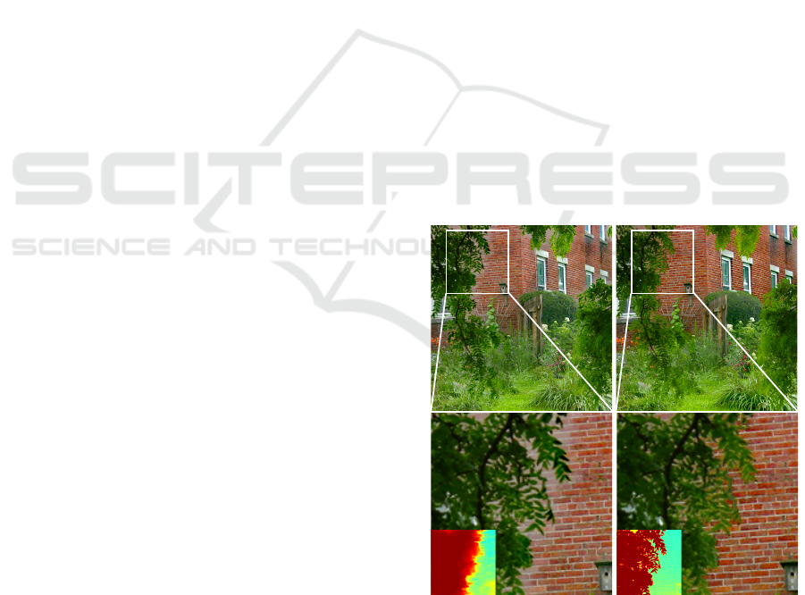
(a) traditional MRF
(b) ours
Figure 1: Comparison of dehazing results using (a) regu-
larization of haze using traditional MRFs commonly used
in most of dehazing algorithms and (b) our regularization
using MRFs with iso-depth NNFs (Insets: corresponding
transmission maps). Our proposed method for single-image
dehazing can propagate haze more effectively than tradi-
tional regularization methods by inferring depth from NNFs
in a hazy image.
Kim I. and H. Kim M.
Dehazing using Non-local Regularization with Iso-depth Neighbor-Fields.
DOI: 10.5220/0006132400770088
In Proceedings of the 12th International Joint Conference on Computer Vision, Imaging and Computer Graphics Theory and Applications (VISIGRAPP 2017), pages 77-88
ISBN: 978-989-758-225-7
Copyright
c
2017 by SCITEPRESS – Science and Technology Publications, Lda. All rights reserved
77

the sparse information to the entire scene to recon-
struct a dense transmittance map, which yields a haze-
free image.
Difficulty of dehazing arises from the existence
of ambiguity due to the lack of the scene informa-
tion. First, the initial assumption on image statis-
tics on natural colors in particular is insufficient to
cover the wide diversity of natural scenes in the real
world, resulting in incomplete haze estimation. No
universal image statistics on natural colors can handle
the dehazing problem. Moreover, as shown in Fig-
ure 1, most of propagation algorithms with a common
grid random field often suffer from haze-isolation ar-
tifacts. The amount of haze in the atmosphere at each
pixel is determined by its depth. In order to handle
abrupt changes of haze density, we need a scene depth
information, even though it is unavailable in single-
image dehazing.
In this paper, we propose a non-local regulariza-
tion for dehazing that can propagate sparse airlight
estimates to yield a dense transmission map with-
out suffering from the typical isolation problem (Fig-
ure 1). Our regularization approach is developed
by combining Markov random fields (MRFs) with
nearest-neighbor fields (NNFs) searched by Patch-
Match (Barnes et al., 2009). Our main insight is
that the NNFs searched in a hazy image associate
patches at the similar depth. Since no depth informa-
tion is available in single-image dehazing, we utilize
the NNFs information to infer depth cues for propa-
gating hidden states of scattered light, which is expo-
nentially proportional to depth (Narasimhan and Na-
yar, 2002). To the best of our knowledge, this ap-
proach is the first work that combines MRF regular-
ization with NNFs for dehazing. This proposed regu-
larization method can be used with any other dehazing
algorithms to enhance haze regularization.
2 RELATED WORK
Previous works on dehazing can be grouped into three
categories: multiple image-based, learning-based,
and single image-based approaches.
Multiple Image-based Dehazing. Since removing
haze in the atmosphere is an ill-posed problem, sev-
eral works have attempted to solve the problem
using multiple input images, often requiring addi-
tional hardware. Schechner et al. capture a set
of linearly polarized images. They utilize the in-
tensity changes of the polarized lights to infer the
airlight layer (Schechner et al., 2001). Narasimhan
et al. employ multiple images with different weather
conditions to restore the degraded image using an
irradiance model (Narasimhan and Nayar, 2002;
Narasimhan and Nayar, 2003). Kopf et al. remove
haze from an image with additionally known scene
geometry, instead of capturing multiple images (Kopf
et al., 2008). These haze formation models stand on
the physics of light transport to provide sound accu-
racy. However, these applications could be limited at
the cost to acquiring multiple input images.
Learning-based Dehazing. Learning-based meth-
ods have been proposed to mitigate the ill-posed
dehazing problem using a trained prior knowledge.
From training datasets, they attempt to earn a prior
on natural image statistics to factorize the haze layer
and the scene radiance from the hazy image. Tang et
al. define haze-relevant features that are related to the
properties of hazy images, and train them using the
random forest regression (Tang et al., 2014). Zhu et
al. obtain the color attenuation prior using supervised
learning (Zhu et al., 2015). They found that the con-
centration of haze is positively correlated with the dif-
ference between brightness and saturation, and they
train a linear model via linear regression. However, no
general statistical model can predict the diverse distri-
butions of natural light environments; hence, they of-
ten fail to restore hazy-free images that are not similar
to the trained dataset.
Single Image-based Dehazing. Owing to the ill-
posedness of the dehazing problem, single image-
based methods commonly rely on a certain assump-
tion on statistics of natural images. Most prior works
have made an assumption on the statistics of natu-
ral scene radiance (Tan, 2008; Tarel and Hauti
`
ere,
2009; He et al., 2009; Nishino et al., 2012; Ancuti
and Ancuti, 2013; Fattal, 2014). Tan and Tarel re-
store visibility by maximizing local contrast, assum-
ing that clean color images have a high contrast, but
this causes overly saturated results (Tan, 2008; Tarel
and Hauti
`
ere, 2009). He et al. exploit image statis-
tics where a natural image in the sRGB color space
should include a very low intensity within a local
region (He et al., 2009). However, it often overes-
timates the amount of haze if there is a large area
having bright pixels. Nishino et al. employ scene-
specific priors, a heavy-tailed distribution on chro-
maticity gradients of colors of natural scenes, to infer
the surface albedo, but they also often produce over-
saturated results (Nishino et al., 2012).
Developing the natural image prior further, Fattal
assumes that in the sRGB space, the color-line of a lo-
cal patch within a clear image should pass through the
origin of the color space (Fattal, 2014). This can yield
a clear and naturally-looking result, but it requires
per-image tweaking parameters such as the gamma
value and the manual estimation of the atmospheric
VISAPP 2017 - International Conference on Computer Vision Theory and Applications
78

light vector. Li et al. suggest a nighttime dehazing
method that removes a glow layer made by the com-
bination of participating media and light source such
as lamps (Li et al., 2015). Recently, a non-local trans-
mission estimation method was proposed by Berman
et al., which is based on the assumption that colors of
a haze-free image can be approximated by a few hun-
dred distinct colors forming tight clusters in the RGB
space (Berman et al., 2016).
In addition, an assumption on light transport in
natural scenes is also used. Fattal assumes that
shading and transmission are statistically indepen-
dent (Fattal, 2008), and Meng et al. impose boundary
conditions on light transmission (Meng et al., 2013).
In particular, our airlight estimation follows the tra-
ditional approach based on dimension-minimization
approach (Fattal, 2008), which allows for robust per-
formance in estimating airlight.
Haze Regularization. Most single-image dehazing
methods estimate per-pixel haze using a patch-wise
operator. Since the operator often fails in a large por-
tion of patches in practice, regularizing sparse haze
estimates is crucial to obtain a dense transmission
map for restoring a haze-free image. Grid Markov
random fields (MRFs) are most commonly used in
many dehazing algorithms (Tan, 2008; Fattal, 2008;
Carr and Hartley, 2009; Nishino et al., 2012; Berman
et al., 2016), and filtering methods are also used, for
instance, matting Laplacian (He et al., 2009), guided
filtering (He et al., 2013), and a total variation-based
approach (Tarel and Hauti
`
ere, 2009; Meng et al.,
2013). These regularization methods only account
for local information, they often fail to obtain sharp
depth-discontinuity along edges if there is an abrupt
change in scene depth.
Recently, Fattal attempts to mitigate this isola-
tion problem by utilizing augmented Markov ran-
dom fields, which extend connection boundaries of
MRFs (Fattal, 2014). However, this method does
not search neighbors in every region in an image
since only pixels within a local window are aug-
mented. For this reason, the augmented MRFs cannot
reflect all non-local information in the image, and in
some cases, isolation artifacts still remain. Berman
et al. non-locally extend the boundary in estimating
haze (Berman et al., 2016); however, they still regu-
larize an initial transmission map by using Gaussian
MRFs (GMRFs) with only local neighbors. As a re-
sult, severe isolation problems occur in a region where
there is an abrupt change of scene depth. In regular-
ization of our method, we extend neighbors in MRFs
with iso-depth NNFs for using additional non-local
information to infer depth cues based on the physics
of light transport.
3 INITIAL ESTIMATION OF
HAZE
We first estimate initial density of haze following a
traditional dimension-reduction approach using lin-
ear subspaces (Narasimhan and Nayar, 2002; Fattal,
2008). To help readers understand the formulation of
the dehazing problem, we briefly provide foundations
of the traditional haze formation model.
Haze Formation Model. Haze is an aerosol that
consists of ashes, dust, and smoke. Haze tends to
present a gray or bluish hue (Narasimhan and Na-
yar, 2002), which leads to decrease of contrast and
color fidelity of the original scene radiance. As the
amount of scattering increases, the amount of degra-
dation also increases. This phenomenon is mathemat-
ically defined as a transmission that represents the
portion of light from the scene radiance that is not
scattered by participating media.
The relationship between the scattered light
and the attenuated scene radiance has been ex-
pressed as a linear interpolation via a transmis-
sion term commonly used in many dehazing algo-
rithms (Narasimhan and Nayar, 2002; Narasimhan
and Nayar, 2003; Fattal, 2008; Fattal, 2014):
I (x) = t (x)J (x) + (1 −t (x))A, (1)
where I(x) is a linearized image intensity
1
at a pixel x,
J(x) is an unknown scene radiance, t(x) is a trans-
mission value, describing the portion of remaining
light when the reflected light from a scene surface
goes to the observer through the medium, and A is
a global atmospheric vector that is unknown as well.
The atmospheric vector A represents the color vector
orientation and intensity of airlight in the linearized
sRGB color space, and along with the interpolation
term (1 −t (x)), the right additive term in Equation (1)
defines the intensity of airlight at the pixel x. Ad-
ditionally, the atmospheric vector is independent of
scene locations, i.e., the atmospheric light is globally
constant.
The number of scattering is closely related to the
distance that light travels, i.e., the longer light trav-
els, the more scattering occurs. Therefore, the trans-
mission decays as light travels. Suppose that haze is
homogeneous; this phenomenon then can be written
as follows: t (x) = e
−βd(x)
, where β is a scattering co-
efficient of the atmosphere (Narasimhan and Nayar,
1
I(x) is linearized by applying a power function with an
exponent of the display gamma to an sRGB value: I(x) =
{I
0
(x)}
γ
, where I
0
(x) is a non-linear RGB value, and γ is
a display gamma (e.g., γ = 2.2 for the standard sRGB dis-
play).
Dehazing using Non-local Regularization with Iso-depth Neighbor-Fields
79

2003) that controls the amount of scattering, and d(x)
is the scene depth at the pixel x.
The goal of haze removal is to estimate transmis-
sion t and an atmospheric vector A so that scene radi-
ance J can be recovered from the transmission t and
the atmospheric vector A by the following:
J (x) =
I (x) − (1 − t (x))A
max(t (x) , ε)
,
where ε is a small value to prevent division by zero.
Haze Estimation. Since airlight is energy scattered
in air, airlight tends to be locally smooth in a scene,
i.e., local airlight remains constant in a similar depth.
In contrast, the original radiance in a scene tend to
vary significantly, naturally showing a variety of col-
ors. When we isolate the scene radiance into a small
patch in an image, the variation of scene radiances
within a patch tends to decrease significantly to form
a cluster with a similar color vector, assuming that
the real world scene is a set of small planar surfaces
of different colors. Then, one can estimate a transmis-
sion value with certain natural image statistics within
a patch based on the local smoothness assumption on
scene depths.
Following this perspective of the traditional ap-
proach (Fattal, 2008), we also define a linear sub-
space that presents local color pixels in the color
space. A linear subspace in each patch comprises
two bases: a scene radiance vector J(x) at the cen-
ter pixel x and a global atmospheric vector A. In this
space, a scene depth is piecewise smooth, and the lo-
cal pixels share the same atmospheric vector. Now
we can formulate dehazing as finding these two un-
known basis vectors, approximating the transmission
value t(x) that is piecewise smooth due to the local
smoothness of a scene depth. Figure 2 depicts the es-
timation process for an overview.
Atmospheric Vector Estimation. Airlight is a
phenomenon that acts like a light source, which is
caused by scattering of participating media in the at-
mosphere (Narasimhan and Nayar, 2002). The atmo-
spheric vector represents the airlight radiance at the
infinite distance in a scene, i.e., the color information
of airlight itself. Therefore, the atmospheric vector
does not include any scene radiance information, and
it only contains the airlight component. The region
full of airlight is the most opaque area in a hazy im-
age. We follow a seminal method of airlight estima-
tion (He et al., 2009). The atmospheric vector A is
estimated by picking up the pixels that have the top
0.1% brightest dark channel pixels and then choosing
the pixel among them that has the highest intensity in
the input image. However, if there are saturated re-
gions such as sunlight or headlights, maximum filter-
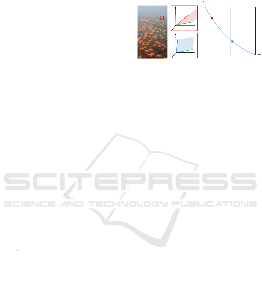
x
(a)
Ω
A
J (x)
R
G
B
()Ix
()I W
I
A
(Ω)
(b)
Transmission estimation
by marginalization
Figure 2: (a) Extracting a patch from a hazy image. I(Ω)
is a set of linearized color pixels in the patch Ω that has a
center pixel of x. The white dot indicates a center pixel x.
(b) We initially estimate the amount of haze using linear
subspaces (Narasimhan and Nayar, 2002; Fattal, 2008). A is
an atmospheric vector of the image (a), I (x) is the linearized
center pixel x depicted as the white dot, and J (x) is the
scene radiance vector of the pixel I (x). The pixel I (x) is
a linear interpolation of the vector A and J (x), and hence
lies on the linear subspace [the blue plane in (b)] spanned
by those two vectors. The red dots describe pixels extracted
from I (Ω). The pixels are projected onto vector A to obtain
a marginal distribution with respect to A. The red arrow
from the cluster denotes the amount of airlight that is deter-
mined from the minimum value of the marginal distribution.
ing of the dark channel could be incorrect since those
regions might have the highest (saturated) dark chan-
nel. Also, we assume that the most opaque region is
the most brightest within an image, and we therefore
discard the pixels that are within aforementioned sat-
urated regions. We then select the 0.1% pixels among
the rest as He et al.’s method does, so that we can
estimate the atmospheric vector consistently. We sub-
sequently average the chosen pixels to reject noise.
Transmission Estimation. We first assume that
transmission is piecewise smooth. In Equation (1),
the portion of haze at a pixel x is determined by the
term (1 − t (x)) that indicates the amount of haze to
be removed. We determine the amount of a haze sig-
nal from given color signals within a patch. Suppose
the given color signals in each patch are linear com-
binations of two unknown bases, J and A, that form
a linear subspace. If we project the given pixels onto
the atmospheric vector A, we can estimate the contri-
bution of the haze signal mixed into the input signals
in the patch.
Supposing I
A
(Ω) is a set of scalar projections of
color vectors I(Ω) onto an atmospheric vector A in
a patch Ω (Figure 2), where the pixel x is located at
the center, then it can be written as following (Fattal,
2008):
I
A
(Ω) = I (Ω) ·
A
k
A
k
, I
A
(Ω) ∈ R
1×
|
Ω
|
.
We assume the airlight within a patch to be constant
VISAPP 2017 - International Conference on Computer Vision Theory and Applications
80
while the scene radiance might vary. In order to focus
only on the airlight component, it is necessary to ob-
tain a marginal distribution of the surrounding pixels
with respect to the basis vector A, as shown in Fig-
ure 2(b).
The marginal distribution I
A
(Ω) describes the his-
togram of airlight components within a patch. This
distribution would have had a very low minimum
value if it had not been influenced by piecewise con-
stant airlight. However, if we take the minimum pro-
jected value, there could be a large chance to take
an outlying value as the minimum. We use the i-th
percentile value from the projected pixel distribution
to reject outliers effectively to achieve robust perfor-
mance:
I
min
A
(Ω) = P
i
k∈Ω
(I
A
(k)) , I
min
A
(Ω) ∈ R
1
,
where P
i
represents an i-th percentile value (i = 2).
The minimum percentile scalar projection onto an
atmospheric vector corresponds to the amount of haze
of a pixel from its patch, and thus the minimum pro-
jection corresponds to the haze component part in
Equation (1), which is (1 − t (x)) ← I
min
A
(Ω).
Additionally, projection onto the atmospheric vec-
tor requires two bases (a pixel and an atmospheric
vectors) to be orthogonal. However, pixels within
a patch are not necessarily orthogonal to the atmo-
spheric vector, so projection needs to be compensated
for non-orthogonality. If a color vector has a small
angle with its atmospheric vector, then its projection
will have a larger value due to the correlation between
the two vectors. We attenuate I
min
A
by a function with
respect to the angle between a pixel vector and an at-
mospheric vector that is given by
t (x) = 1 − f
¯
θ
· I
min
A
(Ω),
where θ is a normalized angle between a pixel vector
and an atmospheric vector within [0,1]. The attenua-
tion function f () is given by
f
¯
θ
=
e
−k
¯
θ
− e
−k
1 − e
−k
, (2)
where the function has a value of [0,1] in the range
of
¯
θ. In this work, we set k = 1.5 for all cases. This
function compensates transmission values by atten-
uating the value I
min
A
since the function has a value
close to 1 if
¯
θ has a small value. See Figure 3(c).
The size of a patch is crucial in our method. If
the size is too small, then the marginal distribution
does not contain rich data from the patch, resulting in
unreliable estimation such as clamping. On the con-
trary, an excessively large patch might include pix-
els in different scene depth and our estimation stage
A
R
G
B
1
J
A
R
G
B
2
J
q
( )
f
q
0.0
0.5
1.0
0.5
1.0
(a) Hazy input (b) Linear subspaces (c) Attenuation function
Figure 3: (a) A hazy input image. (b) Each single pixel
from the red and blue boxes is plotted in the RGB space
along with the atmospheric vector A. J
1
and J
2
in each plot
correspond to the two pixels extracted. (c) The attenuation
function defined as Equation (2) is plotted as above. The
red and blue dots indicate the amount of attenuations of the
red and blue patches. This plot shows that the amount of
attenuation increases as an angle between a color vector and
an atmospheric vector decreases.
takes the minimum value in the marginal distribution,
and hence the transmission estimate will be overes-
timated. In our implementation, we use patches of
15-by-15 pixels and it showed consistent results re-
gardless of the size of an image.
Removing Outliers. While our transmission esti-
mation yields reliable transmission estimates in most
cases, however, there are a small number of cases that
does not obey our assumption. We take them as out-
liers and mark them as invalid transmission values,
and then interpolate them in the regularization stage
(see Section 4).
Distant regions in an image such as sky, and ob-
jects whose color is grayish have a similar color of
haze. In the RGB color space, the angle between an
atmospheric vector and the color vector of a pixel in
those regions is very narrow and the image pixel’s lu-
minance is quite high. In this case, unreliable esti-
mation is inevitable since there is a large ambiguity
between the color of haze and scene radiance. As
a result, unless we do not reject those regions, the
transmission estimate will be so small that those re-
gions will become very dim in turn. For this rea-
son, we discard the transmission estimates, where the
angle between an image pixel and an atmospheric
vector is less than 0.2 radian, the pixel’s luminance
(L
∗
) is larger than 60 in the CIELAB space, and the
estimated transmission value is lower than a certain
threshold: 0.4 for scenes having a large portion of dis-
tant regions and 0.1 for others.
When estimating an atmospheric light, we as-
sumed that the most opaque region in an image is the
brightest area of the whole scene. However, pixels
brighter than the atmospheric light can exist due to
very bright objects such as direct sunlight, white ob-
jects, and lamps in a scene. Those pixels do not obey
our assumption above, and hence this leads to wrong
Dehazing using Non-local Regularization with Iso-depth Neighbor-Fields
81

transmission estimation. Therefore, we discard pixels
whose luminance is larger than the luminance of the
atmospheric light.
4 NON-LOCAL
REGULARIZATION USING
ISO-DEPTH NEIGHBOR
FIELDS
Once we calculate the initial estimates of transmission
for every pixel, we filter out invalid transmission val-
ues obtained from extreme conditions. The transmis-
sion estimation and outlier detection stages might of-
ten yield incomplete results with blocky artifacts. We
therefore need to regularize valid transmission values
in the image.
MRF Model. As we mentioned above, the transmis-
sion is locally smooth. Therefore, in order to obtain
a complete transmission map having sharp-edge dis-
continuities, we need to regularize the incompletely
estimated transmission map using Markov random
fields (MRFs). The probability distribution of one
node in an MRF is given by
p(t (x)
|
ˆ
t (x)) = φ (t (x) ,
ˆ
t (x))ψ(t (x),t (y)), (3)
where t (x) is a latent transmission variable at a
pixel x,
ˆ
t (x) is an initially estimated transmission
value (see Section 3), φ() is a data term of the like-
lihood between t(x) and
ˆ
t(x), and ψ is a smoothness
prior of latent transmission t(x) against neighboring
transmission t(y) within a patch Ω, y ∈ Ω. While the
data term φ() describes the fidelity of observations by
imposing a penalty function between the latent vari-
able and the observed value, the smoothness term ψ()
enforces smoothness by penalizing the errors between
one latent variable and its neighboring variables.
The data term φ() is given by
φ(t (x),
ˆ
t (x)) = exp
−
(t (x) −
ˆ
t (x))
2
σ
ˆ
t
(Ω)
2
!
,
where σ
ˆ
t
(Ω) is the variance of observation values
ˆ
t
within a patch Ω that has the center at a pixel x. See
Figure 4. The data term models error between a vari-
able and observation with in-patch observation vari-
ance noise via a Gaussian distribution. The in-patch
variance of observation values implies that the greater
the variance of in-patch observation is, the more un-
certain the observation values are, resulting in giving
less influence from the data term on the distribution.
The smoothness term Ψ() is written as
ψ(t (x),t (y)) =
∏
y∈N
x
exp
−
(t (x) − t (y))
2
k
I (x) − I (y)
k
2
!
,
where I () is a linearized pixel intensity of an image,
and pixel y is in a set of neighbors N
x
of pixel x. The
smoothness term encourages smoothness among one
variable and its neighboring variables by penalizing
pairwise distances between them, where the distribu-
tion of the distances follows a Gaussian distribution.
If (t (x) −t (y))
2
is large, then it indicates that the dis-
tance between t (x) and its neighbor t (y) is large, and
hence the cost from the regularization term will also
become large, which enforces strong smoothness be-
tween them.
k
I (x) − I (y)
k
2
in the denominator of the
prior term controls the amount of smoothness by ex-
ploiting information from an input image. This prop-
erty implies that if two image pixels are similar, then
their transmission values are likely to be similar as
well. On the contrary, it gives sharp-edge discontinu-
ity in transmission values along edges since the value
of the denominator becomes large when the difference
between two pixels is large.
In fact, the probability distribution of an MRF
over the latent variable t is modeled via a Gaus-
sian distribution. In this case, the MRF is formal-
ized by using a Gauss-Markov random field (GMRF),
which can be solved by not only using computation-
ally costly solvers, but also by a fast linear system
solver (Marroqu
´
ın et al., 2001; Fattal, 2008).
Finally, we formulate a cost function by taking
the negative log of the posterior distribution [Equa-
tion (3)] following (Fattal, 2008; Fattal, 2014), which
is written by
E (t) =
∑
x
(
(t (x) −
ˆ
t (x))
2
σ
ˆ
t
(Ω)
2
+
∑
y∈N
x
(t (x) −t (y))
2
k
I (x) − I (y)
k
2
)
.
The regularization process is done by minimizing
the cost function, which is solved by differentiating
the function with respect to t and setting it to be zero.
Iso-depth Neighbor Fields. In conventional grid
MRFs, a prior term (smoothness term in this text) as-
sociates adjacent four pixels as neighbors for regular-
ization. However, pixels in a patch lying on an edge
may be isolated when the scene surface has a com-
plicated shape. In Figure 4(a), the leaves in the left
side of the image have a complicated pattern of edges,
and the bricks lie behind the leaves. If we model a
grid MRF on the image, then pixels on the tip of the
leaves will be isolated by the surrounding brick pix-
els. In this case, smoothness of the leaf pixels will
be imposed mostly by the brick pixels, where there
is a large depth discontinuity between them. In other
words, a large scene depth discrepancy exists in the
patch, and thus if some pixels lying on the edge are
only connected to their adjacent neighbors, the prior
term will enforce wrong smoothness due to the large
depth discrepancy. As a result, those regions will be
VISAPP 2017 - International Conference on Computer Vision Theory and Applications
82
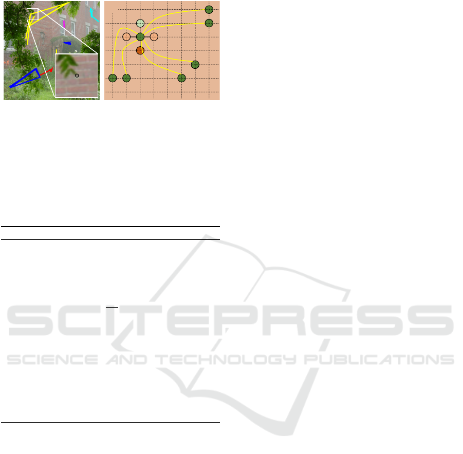
(a) (b)
x
x
W
Figure 4: (a) The picture shows some sampled NNFs that
associate pixels having similar scene depths. The line with
the same color denotes association of pixels in the same
NNF. (b) An MRF model of the node x from the patch in (a)
associated with adjacent four neighbors and distant neigh-
bors in the NNF. Since the node x is located in the end point
of the leaf, its adjacent pixels have very different transmis-
sion values due to a large depth discontinuity. As (a) shows,
the neighbors connected with the same NNF have very sim-
ilar scene depths, and hence they give a more accurate reg-
ularization cue than the adjacent neighbors do.
Algorithm 1: Dehazing via Non-Local Regularization.
Require: an image I
Ensure: a result image J and a transmission map t
1:
ˆ
A ← ATMOSPHERICVECTORESTIMATE(I)
2:
{
I
L
,A
}
← INVERSEGAMMACORRECT(
I,
ˆ
A
)
3: for pixels x = 1 to n do
4: I
A
(Ω) ← I
L
(Ω) ·
A
k
A
k
5: I
min
A
(Ω) ← P
i
k∈Ω
(I
A
(k))
6: t
0
(x) ← 1 − f
¯
θ
· I
min
A
(Ω)
7:
ˆ
t (x) ← OUTLIERREJECT(t
0
(x), A, I
L
(x))
8: end for
9: NNF ← PATCHMATCH(I)
10: t ← REGULARIZE(NNF,
ˆ
t,I)
11: J
L
← (I − (1 −t)A)/t
12: J ← GAMMACORRECT(J
L
)
overly smoothed out due to the wrong connection of
neighbors.
While Besse et al. use the PatchMatch algo-
rithm (Barnes et al., 2009) to rapidly solve non-
parametric belief propagation (Besse et al., 2014),
we investigate neighbors extracted from a nearest-
neighbor field (NNF) using the PatchMatch algorithm
and found that the NNF associates pixels at simi-
lar scene depths. This insightful information gives a
more reliable regularization penalty since the neigh-
boring nodes in the NNF are likely to have similar
transmission estimates. Thus, we add more neighbors
belonging to the same NNF to the smoothness term
and perform statistical inference on the MRF along
with them. We note that these long-range connections
in regularization are desirable in many image process-
ing applications, addressed by other works (Fattal,
2014; Li and Huttenlocher, 2008). After regulariza-
tion, we use the weighted median filter (Zhang et al.,
2014) to refine the transmission map. Algorithm 1
summarizes our dehazing algorithm as an overview.
5 RESULTS
We implemented our algorithm in a non-optimized
MATLAB environment except the external Patch-
Match algorithm (Barnes et al., 2009), and processed
it on a desktop computer with Intel 4.0 GHz i7-
4790K CPU and 32 GB memory. For the case of the
house image of resolution 450 × 440 shown in Fig-
ure 1(b), our algorithm took 6.44 seconds for running
the PatchMatch algorithm to seek 17 neighbors, 8.32
seconds to estimate an atmospheric vector, transmis-
sion values and rejecting outliers, 43.43 seconds for
our regularization stage, and 0.65 seconds for running
the weighted median filter and recovering the scene
radiance, taking approximately 58.84 seconds in to-
tal. We evaluated our algorithm with a large number
of outdoor hazy images obtained from (Fattal, 2014)
to prove robustness, and we also present comparisons
with state-of-the-art dehazing methods. Refer to the
supplemental materials for more results.
Regularization. We compare results of our method
with those of state-of-the-art methods in terms of reg-
ularization. Berman et al. regularize initial transmis-
sion estimates with a grid GMRF as shown in third
and fourth columns in Figure 5 (Berman et al., 2016).
Due to the lack of non-local information in regular-
ization, certain regions suffer from the haze isolation
problem as mentioned above. Other than using a grid
MRF, Fattal takes an augmented GMRF model for
regularization, which extends neighbor fields within
a local window (Fattal, 2014). However, it does not
connect more neighbors for all pixels due to time
complexity. As a result, certain regions are not fully
recovered from the haze isolation problem. Figure 5
validates that our method successfully removes haze
even from a scene having abrupt depth changes with
complicated patterns.
Figure 6 shows the intermediate stages in our reg-
ularization process of transmission (d) – (g), along
with our result of the house scene (c). We start our
regularization from Figure 6(d) that has outliers [rep-
resented as black pixels in Figure 6(d)]. In par-
ticular, Figures 6(e) and (f) compare the impact of
NNFs in the MRF regularization. When we reg-
ularize the initial estimate with only GMRFs, cer-
tain regions with complex scene structures are over-
smoothed due to the wrong smoothness penalty as
Figure 6(e) shows. We account for additional neigh-
Dehazing using Non-local Regularization with Iso-depth Neighbor-Fields
83
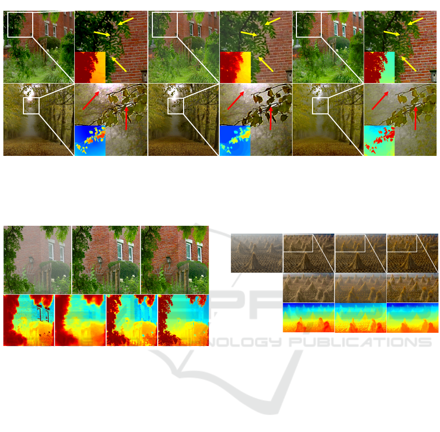
Fattal14 ours
Berman et al.close-up
close-up
close-up
Figure 5: Comparisons of dehazing in terms of regularization. The four columns from left are results from other two meth-
ods: (Fattal, 2014) using augmented GMRFs and (Berman et al., 2016) using traditional GMRFs, and the last fifth and sixth
columns are our results (Insets: corresponding transmission maps). While other methods often fail to obtain sharp edge-
discontinuities in the images, our method yields clear recovered scene radiance maps as shown above. Notable regions are
pointed with arrows.
(a) (b)
(c)
(d) (e) (f) (g)
Figure 6: We present an example before and after applying
our dehazing and regularization method. (a) The hazy in-
put image. (b) The recovered scene radiance map with the
transmission map regularized by grid MRFs (e). (c) The
recovered scene radiance map with the final transmission
map (g). Images (d) – (g) compare transmission maps to
show the influence of using iso-depth NNFs. All regular-
izations are done using GMRFs. (d) The initial transmis-
sion estimates including discarded pixels (the black pix-
els). (e) The regularized transmission map without NNFs.
(f) The regularized transmission map with NNFs. (g) The
final refined map of (f) using the weighted median filter.
bors from NNFs to obtain a clearer transmission map
shown in Figure 6(f). Figure 6(g) shows the final
transmission map that we refine with a weighted me-
dian filter (Zhang et al., 2014).
We also compare our regularization method with
representative matting methods: the matting Lapla-
cian method (Levin et al., 2008) and the guided fil-
ter method (He et al., 2013) in Figure 7. While we
use the guide image as just a guide to smooth and en-
force sharp gradient along edges on transmission es-
timates, both methods are based on the assumption
that an output and an input guidance form a linear
original guided filter
matting Laplacian
ours
dehazed
(close-up)
transmission
(close-up)
Figure 7: We compare our regularization with other meth-
ods. The leftmost one is the original image of cones. The
first row shows dehazed results with our transmission esti-
mation step and each regularization method written at the
lower right. We cropped the dehazed images in the first row
to highlight the influence of regularization methods in the
second row. The third row presents a sequence of cropped
transmission maps in the same manner as the second row.
relationship. As described in Section 3, scene radi-
ance varies largely while transmission does the oppo-
site. Consequently, the two methods follow the be-
havior of the scene radiance, which results in distort-
ing the given estimates. As a result, our regulariza-
tion method yields an accurate transmission map with
clear-edge discontinuities while the others overesti-
mate the transmission estimates in turn.
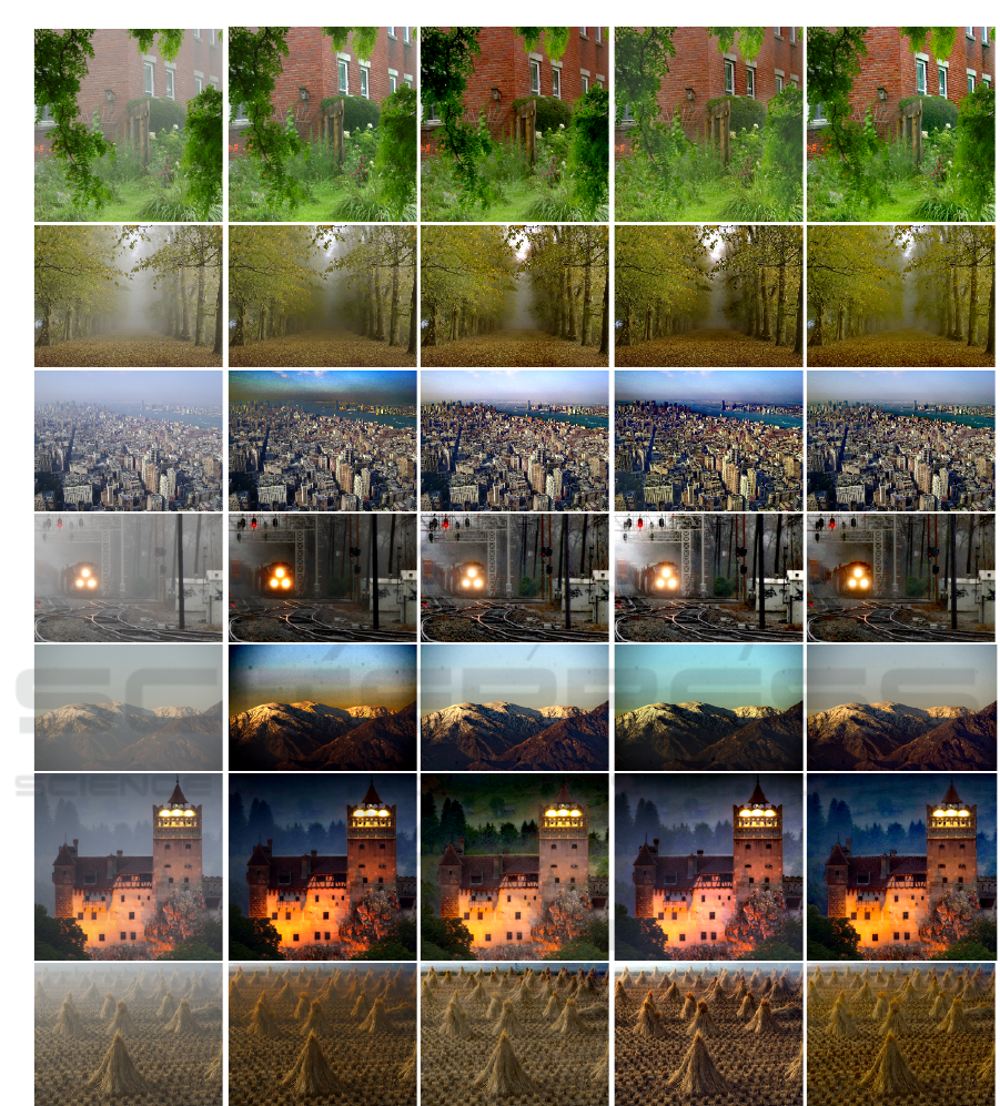
Qualitative Comparison. Figure 8 qualitatively
validates the robust performance in dehazing the com-
mon reference dataset of hazy scenes (Fattal, 2014).
We compare the performance of our dehazing algo-
rithm with three state-of-the-art methods (He et al.,
2009; Fattal, 2014; Berman et al., 2016). We were
motivated to achieve consistent performance of de-
hazing with less parameter controls like other im-
VISAPP 2017 - International Conference on Computer Vision Theory and Applications
84
He et al.
Fat t al14
ours
Berman et al.
houseforestny17train
cones
snow
castle
input
Figure 8: Validation of consistency of dehazing. The first column shows input images. The second, third, and fourth columns
are results from (He et al., 2009; Fattal, 2014; Berman et al., 2016), respectively. The fifth column presents our method’s
results. We use the set of parameters as described in Section 3. For the images in the third and fifth rows, we only set
the threshold of lower bound transmission to 0.4 and the others to 0.1 for removing narrow angle outliers. Our method is
competitive to other method (Fattal, 2014) that requires with manual tweaking parameters to achieve plausible results. Refer
to the supplemental material for more results.
age processing algorithms (Kim and Kautz, 2008;
Kim and Kautz, 2009). Figure 8 shows results us-
ing the single set of parameters as described in Sec-
tion 3. Our method shows competitive results to other
method (Fattal, 2014) that requires manual tweaking
parameters per scene to achieve plausible results. For
close-up images of the results, refer to the supplemen-
tal material.
Time Performance. Table 1 compare the compu-
tational performance of our method with traditional
Dehazing using Non-local Regularization with Iso-depth Neighbor-Fields
85
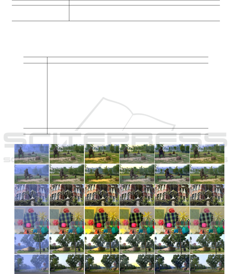
Table 1: Comparison of time performance of dehazing with the traditional grid GMRFs and our GMRFs with iso-depth NNFs
(unit: second). Refer to Figure 8 for processed images. The third row shows computational costs of only seeking NNFs with
17 neighbors using PatchMatch (Barnes et al., 2009) in our method.
Dehazing house forest ny17 train snow castle cones average
with grid GMRFs 6.43 26.55 27.51 7.74 18.88 12.84 6.41 15.19
with NNF-GMRFs 58.84 305.48 305.06 73.06 191.76 129.18 61.12 160.64
(for computing NNFs only) (6.44) (31.82) (28.48) (7.15) (18.54) (11.01) (7.31) (15.82)
Table 2: Quantitative comparisons of our method with other methods (He et al., 2009; Fattal, 2014; Berman et al., 2016).
The error values are computed from the entire synthetic hazy image dataset provided by (Fattal, 2014). All figures represent
mean L
1
error of the estimated transmission t (left value) and output image J (right value). Red figures indicate the best
results, and blue for the second best. For a fair comparison, parameters for each method, such as display gamma for sRGB
linearization and the airlight vector, were optimized for the highest performance.
(He et al., 2009) (Fattal, 2014) (Berman et al., 2016) ours
church 0.0711/0.1765 0.1144/0.1726 0.1152/0.2100 0.1901/0.1854
couch 0.0631/0.1146 0.0895/0.1596 0.0512/0.1249 0.0942/0.1463
flower1 0.1639/0.2334 0.0472/0.0562 0.0607/0.1309 0.0626/0.0967
flower2 0.1808/0.2387 0.0418/0.0452 0.1154/0.1413 0.0570/0.0839
lawn1 0.1003/0.1636 0.0803/0.1189 0.0340/0.1289 0.0604/0.1052
lawn2 0.1111/0.1715 0.0851/0.1168 0.0431/0.1378 0.0618/0.1054
mansion 0.0616/0.1005 0.0457/0.0719 0.0825/0.1234 0.0614/0.0693
moebius 0.2079/0.3636 0.1460/0.2270 0.1525/0.2005 0.0823/0.1138
reindeer 0.1152/0.1821 0.0662/0.1005 0.0887/0.2549 0.1038/0.1459
road1 0.1127/0.1422 0.1028/0.0980 0.0582/0.1107 0.0676/0.0945
road2 0.1110/0.1615 0.1034/0.1317 0.0602/0.1602 0.0781/0.1206
average 0.1181/0.1862 0.0839/0.1180 0.0783/0.1567 0.0836/0.1152
lawn1
He et al. Fattal14 Berman et al. oursground truth
mansionmoebius
road1 lawn2
road2
hazy input
Figure 9: Dehazed results for the quantitative comparison shown in Table 2. The first column shows synthetic hazy images
generated from the ground truth dataset (Fattal, 2014) in the second column with their corresponding depth maps. The
remaining columns are recovered scene radiance maps by each method. Our method yields consistent results compared with
other methods. Parameters for each method were optimized for the highest performance for a fair comparison.
VISAPP 2017 - International Conference on Computer Vision Theory and Applications
86
original
29×29
3×3
15×15
(a) (b)
(c)
(d)
Figure 10: Comparisons to show the influence of a patch
size in estimating transmission. (a) The original canon im-
age. (b) The dehazed image with a patch size of 3×3 where
severe color clamping happens. (c) The dehazed image with
a patch size of 15×15, which is our choice for all results. (d)
The dehazed image with a patch size of 29×29 in which the
airlight in distant regions is underestimated.
grid GMRFs and our iso-depth GMRFs using images
shown in Figure 8. We also shows computational
costs of obtaining only NNFs with 17 neighbors using
PatchMatch (Barnes et al., 2009) in the third row. De-
hazing with iso-depth NNF-GMRFs takes 10.58 times
more time; however, iso-depth NNFs give richer in-
formation in regularization, resulting in more exact
scene radiance recovery.
Quantitative Comparison. We compare our
method with the entire synthetic hazy image dataset
provided by (Fattal, 2014). The synthetic hazy images
were generated by datasets that contain clear indoor
and outdoor scenes, and their corresponding depth
maps. Table 2 reports the quantitative comparison of
our method with other methods (He et al., 2009; Fat-
tal, 2014; Berman et al., 2016). We also show the
dehazed images used for the quantitative comparison
in Figure 9. Our method shows competitive and con-
sistent results particularly in dehazed images.
Impact of Patch Size. Figure 10 shows the results
of dehazing under varying patch sizes. Image (a) is an
input image of canon, the size of which is 600 × 524.
Image (b) is severely over-saturated since the size of
patches is so small that each patch cannot contain
rich information of scene structures, i.e., the patch
failed to reject the influence of highly-varying nature
of scene radiance. On the other hand, as shown in
image (d), its airlight is underestimated since patches
are too large to hold the assumption that transmis-
sion is piecewise constant. This underestimation is
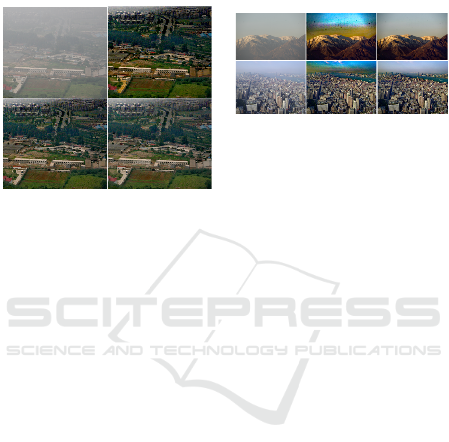
input
without rejection
with rejection
Figure 11: Validation of our narrow angle outlier rejection
method described in Section 3. In the second column, the
distant region represented as sky has an infinite depth, and
hence our transmission estimation stage estimates its trans-
mission as being close to zero, which yields overly saturated
results. We obtained consistent results by our outlier rejec-
tion stage, as shown in the third column.
exacerbated in distant regions where their scene depth
changes rapidly. In our experiment, we found that the
patch size of 15×15 works properly for most scenes,
and therefore we take the same patch size for all re-
sults in this paper.
Outlier Removal. We validate our outlier-rejection
process. Figure 11 shows the regions in infinite scene
depths occupy a large portion of the image that is full
of airlight in the two input images. In these regions,
there is a large ambiguity between airlight and scene
radiance, and hence our method fails to produce a nat-
urally looking result as the second column shows. Af-
ter we discard outliers having a narrow angle between
the atmospheric vector and the input color pixel, we
could obtain high-quality scene radiance maps in the
third column.
6 CONCLUSION
We have presented a dehazing algorithm using non-
local regularization with iso-depth neighbor fields.
Even though regularization is an essential process
in dehazing, traditional GMRF-based regularization
methods often fail with isolation artifacts when there
is an abrupt change in depth, of which information
is missing in single-image dehazing. We propose
a novel non-local regularization method that utilizes
NNFs searched in a hazy image to infer depth cues
to obtain more reliable smoothness penalty for han-
dling the isolation problem in dehazing. We validated
the robust performance of our method with extensive
test images and compared it with the state-of-the-art
single image-based methods. This proposed regular-
ization method can be used separately with any other
dehazing algorithms to enhance haze regularization.
Dehazing using Non-local Regularization with Iso-depth Neighbor-Fields
87

ACKNOWLEDGMENTS
Min H. Kim, the corresponding author, gratefully ac-
knowledges Korea NRF grants (2016R1A2B2013031
and 2013M3A6A6073718) and additional support by
an ICT R&D program of MSIP/IITP (B0101-16-
1280). We also would like to appreciate Seung-Hwan
Baek’s helpful comments.
REFERENCES
Ancuti, C. O. and Ancuti, C. (2013). Single image dehazing
by multi-scale fusion. IEEE Trans. Image Processing,
22(8):3271–3282.
Barnes, C., Shechtman, E., Finkelstein, A., and Goldman,
D. B. (2009). Patchmatch: a randomized correspon-
dence algorithm for structural image editing. ACM
Trans. Graph, 28(3):24:1–24:11.
Berman, D., Treibitz, T., and Avidan, S. (2016). Non-local
image dehazing. In IEEE CVPR, pages 1674–1682.
Besse, F., Rother, C., Fitzgibbon, A. W., and Kautz, J.
(2014). PMBP: Patchmatch belief propagation for
correspondence field estimation. International Jour-
nal of Computer Vision, 110(1):2–13.
Carr, P. and Hartley, R. I. (2009). Improved single image
dehazing using geometry. In DICTA 2009, pages 103–
110.
Fattal, R. (2008). Single image dehazing. ACM Trans.
Graph., 27(3):72:1–72:9.
Fattal, R. (2014). Dehazing using color-lines. ACM Trans.
Graph., 34(1):13:1–13:14.
He, K., Sun, J., and Tang, X. (2013). Guided image filtering.
IEEE Trans. Pattern Anal. Mach. Intell., 35(6):1397–
1409.
He, K. M., Sun, J., and Tang, X. (2009). Single image
haze removal using dark channel prior. In Proc. IEEE
CVPR, pages 1956–1963.
Kim, M. H. and Kautz, J. (2008). Consistent tone reproduc-
tion. In Proc. the IASTED International Conference
on Computer Graphics and Imaging (CGIM 2008),
pages 152–159, Innsbruck, Austria. IASTED/ACTA
Press.
Kim, M. H. and Kautz, J. (2009). Consistent scene illumi-
nation using a chromatic flash. In Proc. Eurographics
Workshop on Computational Aesthetics (CAe2009),
pages 83–89, British Columbia, Canada. Eurograph-
ics.
Kopf, J., Neubert, B., Chen, B., Cohen, M. F., Cohen-
Or, D., Deussen, O., Uyttendaele, M., and Lischin-
ski, D. (2008). Deep photo: model-based photo-
graph enhancement and viewing. ACM Trans. Graph.,
27(5):116:1–116:10.
Levin, A., Lischinski, D., and Weiss, Y. (2008). A closed-
form solution to natural image matting. IEEE Trans.
Pattern Anal. Mach. Intell., 30(2):228–242.
Li, Y., Tan, R. T., and Brown, M. S. (2015). Nighttime haze
removal with glow and multiple light colors. In 2015
IEEE ICCV 2015, Santiago, Chile, December 7-13,
2015, pages 226–234.
Li, Y. P. and Huttenlocher, D. P. (2008). Sparse long-range
random field and its application to image denoising.
In ECCV, pages III: 344–357.
Marroqu
´
ın, J. L., Velasco, F. A., Rivera, M., and Nakamura,
M. (2001). Gauss-markov measure field models for
low-level vision. IEEE Trans. Pattern Anal. Mach.
Intell., 23(4):337–348.
Meng, G., Wang, Y., Duan, J., Xiang, S., and Pan, C.
(2013). Efficient image dehazing with boundary con-
straint and contextual regularization. In Proc. IEEE
ICCV, pages 617–624.
Narasimhan, S. G. and Nayar, S. K. (2002). Vision and
the atmosphere. Int. Journal of Computer Vision,
48(3):233–254.
Narasimhan, S. G. and Nayar, S. K. (2003). Contrast
restoration of weather degraded images. IEEE Trans.
Pattern Anal. Mach. Intell, 25(6):713–724.
Nishino, K., Kratz, L., and Lombardi, S. (2012).
Bayesian defogging. Int. Journal of Computer Vision,
98(3):263–278.
Schechner, Y. Y., Narasimhan, S. G., and Nayar, S. K.
(2001). Instant dehazing of images using polarization.
In Proc. IEEE CVPR, pages I:325–332.
Tan, R. T. (2008). Visibility in bad weather from a single
image. In Proc. IEEE CVPR, pages 1–8.
Tang, K., Yang, J., and Wang, J. (2014). Investigating haze-
relevant features in a learning framework for image
dehazing. In Proc. IEEE CVPR, pages 2995–3002.
Tarel, J. and Hauti
`
ere, N. (2009). Fast visibility restoration
from a single color or gray level image. In Proc. IEEE
ICCV, pages 2201–2208.
Zhang, Q., Xu, L., and Jia, J. (2014). 100+ times faster
weighted median filter (WMF). In CVPR, pages
2830–2837. IEEE.
Zhu, Q., Mai, J., and Shao, L. (2015). A fast single image
haze removal algorithm using color attenuation prior.
IEEE Trans. Image Processing, 24(11):3522–3533.
VISAPP 2017 - International Conference on Computer Vision Theory and Applications
88
