Pushing the Limits for View Prediction in Video Coding
Jens Ogniewski and Per-Erik Forss
´
en
Department of Electrical Engineering, Link
¨
oping University,
581 83 Link
¨
oping, Sweden
{jenso, perfo}@isy.liu.se
Keywords:
Projection Algorithms, Video Coding, Motion Estimation.
Abstract:
More and more devices have depth sensors, making RGB+D video (colour+depth video) increasingly com-
mon. RGB+D video allows the use of depth image based rendering (DIBR) to render a given scene from
different viewpoints, thus making it a useful asset in view prediction for 3D and free-viewpoint video coding.
In this paper we evaluate a multitude of algorithms for scattered data interpolation, in order to optimize the
performance of DIBR for video coding. This also includes novel contributions like a Kriging refinement step,
an edge suppression step to suppress artifacts, and a scale-adaptive kernel. Our evaluation uses the depth ex-
tension of the Sintel datasets. Using ground-truth sequences is crucial for such an optimization, as it ensures
that all errors and artifacts are caused by the prediction itself rather than noisy or erroneous data. We also
present a comparison with the commonly used mesh-based projection.
1 INTRODUCTION
With the introduction of depth sensors on mobile de-
vices, such as the Google Tango, Intel RealSense
Smartphone, and HTC ONE M8, RGB+D video is
becoming increasingly common. There is thus an in-
terest to incorporate efficient storage and transmission
of such data into upcomingvideo standards.
RGB+D video data enables depth image based ren-
dering (DIBR) which has many different applications
such as frame interpolation in rendering (Mark et al.,
1997), and rendering of multi-view plus depth (MVD)
content for free viewpoint and 3D display (Tian et al.,
2009).
In this paper, we investigate the usage of DIBR to do
view prediction (VP) for video coding. To find out
how well VP can perform, we examine how much
DIBR can be improved using modern scattered data
interpolation techniques.
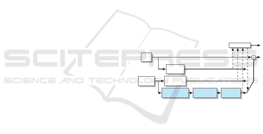
Current video standards such as HEVC/H.265 use
block based motion vector compensation. When a
depth stream is available, VP can also be incorpo-
rated to predict blocks from views generated through
DIBR, see figure 1. A DIBR frame is often a better
approximation of the frame to be encoded than pre-
vious or future frames. Thus, VP can improve the
prediction.
View prediction for block based coding has pre-
viously been explored using mesh-based projection
(also known as texture mapping) (Mark et al., 1997;
Coder control
Input
frame
Reference
frame(s)
Intra-frame
prediction
Motion
compensation
Occlusion aware
projection
Scattered data
interpolation
Hole-filling/
Inpainting
Figure 1: Overview of the suggested prediction unit of a
predictive video coder
Light-blue boxes at the bottom are view-prediction addi-
tions to the conventional pipeline, the parts treated in this
paper use bold font.
Shimizu et al., 2013) and the closely related inverse
warp (interpolation in the source frame) (Morvan
et al., 2007; Iyer et al., 2010). These studies demon-
strate that even very simple view prediction schemes
give coding gains. In this paper we try to find the
limits of VP by comparing mesh-based projection
with more advanced scattered data interpolation tech-
niques.
Scattered data interpolation in its most simple form
uses a form of forward warp called splatting (Szeliski,
2011) to spread the influence of a source pixel. While
forward warping is often more computationally ex-
pensive than mesh-based projection, and risks leav-
ing holes in the output image as a change of view can
cause self occlusions (Iyer et al., 2010), it can also
lead to higher preservation of details. An enhance-
68
Ogniewski J. and ForssÃl’n P.
Pushing the Limits for View Prediction in Video Coding.
DOI: 10.5220/0006131500680076
In Proceedings of the 12th International Joint Conference on Computer Vision, Imaging and Computer Graphics Theory and Applications (VISIGRAPP 2017), pages 68-76
ISBN: 978-989-758-225-7
Copyright
c
2017 by SCITEPRESS – Science and Technology Publications, Lda. All rights reserved

ment of splatting is agglomerative clustering (AC)
(Mall et al., 2014; Scalzo and Velipasalar, 2014),
where subsets of points are clustered (in color and
depth) and merged. This step implements the oc-
clusion aware projection box shown in figure 1. Fi-
nally, even more details can be preserved by taking
the anisotropy of the texture into account, using Krig-
ing (Panggabean et al., 2010; Ringaby et al., 2014).
Note that many of these methods have not been ap-
plied in DIBR before.
When a part of the target frame is occluded in all
input frames, there will be holes in the predicted
view. Blocks containing holes can be encoded us-
ing conventional methods (without any prediction in
the worst case). Alternatively, a hole-filling algorithm
can be applied, e.g. hierarchical hole-filling (HFF)
(Solh and Regib, 2010). This is especially recom-
mended for small holes, to allow an efficient predic-
tion from these blocks. Here, we do not compare
different hole-filling approaches; instead we limit the
evaluation to regions that are visible (see the masks
in figure 2), and use our own, enhanced implementa-
tion of HFF (Solh and Regib, 2010) to fill small holes
when needed.
We use the depth extension of the Sintel datasets (But-
ler et al., 2012) for tuning and evaluation, see figure
3. These provide ground-truth for RGB, depth and
camera poses.
2 PROJECTION METHODS
In order to find an overall optimal solution, we inte-
grated a multitude of different methods and param-
eters in a flexible framework which we tuned using
training data. This framework includes both state-of-
the-art methods (e.g. agglomerative clustering, Krig-
ing) as well as own contributions (a Kriging refine-
ment step, an edge suppression step to suppress arti-
facts, and a scale-adaptive kernel).
In the following, we will describe the different param-
eters and algorithms used by our forward-warping so-
lution.
2.1 Global Parameters
Global parameters are parameters that influence all of
the different algorithms. We introduced the possibil-
ity to work on an upscaled image internally (by a fac-
tor S
u
in both width and height), and also a switch to
use either square or round convolution kernels in all
methods that are applied on a neighborhood.
We also noticed that a fixed kernel size performed
suboptimally, as view changes can result in a scale
change that varies with depth. For objects close to
the camera, neighboring pixels in the source frame
may end up many pixels apart in the target frame. If
the kernel is too small, pixels in-between will not be
reached by the kernel, giving the object a “shredded”
look (see also figure 5, especially the yellow rectangle
in the image at the bottom).
To counter these effects, we introduce an adaptive
splat kernel, adjusted to the local density of pro-
jected points. This is a generalization of ideas found
in (Ringaby et al., 2014), where the shape of the
region is defined for the application of an aircraft-
mounted push-broom camera. Here we generalize
this by instead estimating the shape from neighbor-
ing projected points:
For each candidate point, we calculate the distances
between its projected position in the output image and
the projected positions of its eight nearest neighbors
in the input image. The highest distances in x and y
directions are then used to define the splatting rect-
angle. This is made more robust by a simple outlier
rejection scheme: each distance d
k
is compared to the
smallest distance found in the neighborhood, and if
this ratio is above a threshold T
reldist
this neighbor is
ignored in the calculation of the rectangle. This out-
lier rejection is done to handle points on the edge of
objects. Note that this simple scheme assumes an ob-
ject curvature that is more or less constant in all di-
rections, and will remove too many neighbors if this
is not the case.
2.2 Candidate Point Merging
In our forward warp, each pixel of an input image is
splatted to a neighborhood in the output image. Thus,
a number of input pixels are mapped to the same out-
put pixel, so called candidates, which are merged us-
ing a variant of agglomerative clustering. First, we
calculate a combined distance in depth and color be-
tween all candidates:
d = d
RGB
W
c
+ d
DEPTH
, (1)
where W
c
is a parameter to be tuned. We then merge
the two that have the lowest distance to each other,
then recalculate the distances and merge again the
two with the lowest distance. We use a weighted
average to merge the pixels, where the initial weights
come from a Gaussian kernel:
g
p−p
0
= exp(−W
k
||diag(1/w
x
,1/w
y
)(p − p
0
)||) (2)
Here p is the projected pixel position, and p
0
is the
position of the pixel we are currently coloring. Fur-
ther w
x
and w
y
are the maximal kernel-sizes in x and
Pushing the Limits for View Prediction in Video Coding
69
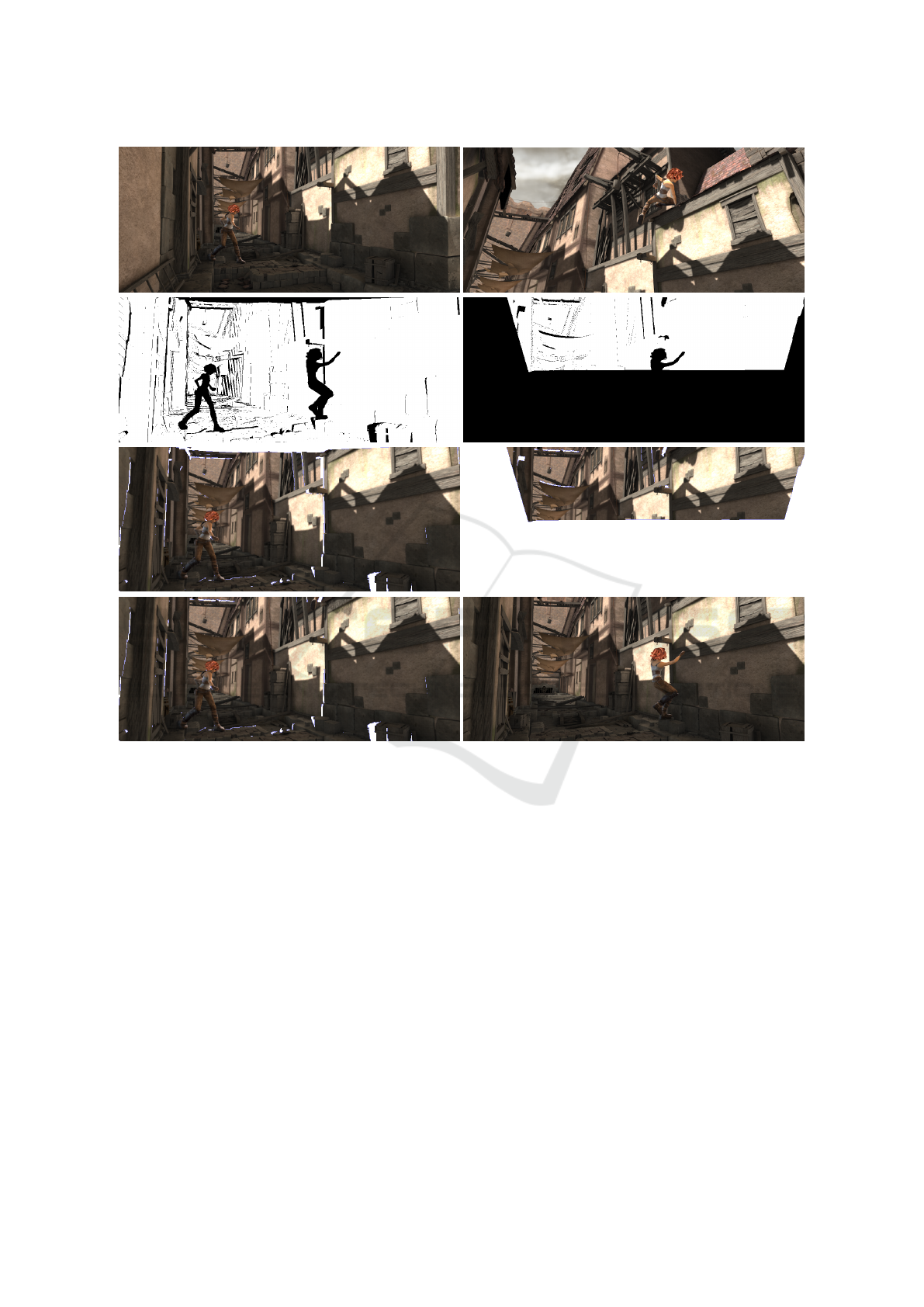
Figure 2: Example from one of the two tuning sequences:
Top row: input images, image 1 (left) and image 49 (right).
2nd row: mask images used in PSNR calculation for target frame 25, for projection of image 1 (left), and image 49 (right).
3rd row: view prediction from image 1 (left), and image 49 (right).
Bottom row: both predictions combined (left), and ground-truth frame 25 (right).
y directions, used during splatting the output pixel in
question (these are constant if scale adaptive splatting
is switched off), and W
k
is a parameter to be tuned.
The euclidean norm is used. The accumulated weight
of the merged candidate is calculated by adding their
weights, to give merged candidates containing more
contributions a higher We repeat this step until the
lowest distance between the candidate points is higher
than a tuned threshold T
ACmax
, and select the merged
cluster with the highest score based on its (accumu-
lated) weight w
p
and its depth d
p
(i.e. distance to the
camera):
s = w
p
W
a
+ 1/d
p
, (3)
where W
a
is a blending parameter to be tuned. Note
that regular splatting is a special case of this method
which can be obtained by setting both W
c
and W
a
to 0.
2.3 Kriging
We also tested Kriging (Panggabean et al., 2010;
Ringaby et al., 2014) as a method to merge the can-
didates. In Kriging, the blending weight calculation
described earlier is replaced by a best linear unbiased
estimator using the covariance matrix of different
samples in a predetermined neighborhood. While
isotropic Kriging is based solely on the distances of
the samples to each other, anistropic Kriging takes
also the local gradients into account, and can thus be
seen as fitting a function of a higher degree. After
adding a new candidate to a cluster, its new values
VISAPP 2017 - International Conference on Computer Vision Theory and Applications
70

are calculated using the original input data of all
candidates it contains.
However, due to camera rotation and pan-
ning/zooming motions, these gradients might
differ to the ones found in the projected images.
Thus, we also included Kriging as a refinement step,
in which candidate merging and selection is repeated
using anisotropic Kriging, and the gradients are
calculated based on the projected image rather than
the input images.
2.4 Image Merging
Projecting from several images, the different pro-
jected images need to be merged to a final one. For
this, again agglomerative clustering as described ear-
lier was used, where the candidates are the pixels in
the different images at a fixed position, rather than a
neighborhood.
In the merging process, all weights were multiplied
with a frame distance weight, giving samples close in
time a higher blend weight.
We found that the smooth transitions (anti-aliased
edges) in the textures of the input frames lead to un-
wanted artifacts (see also figure 5). To counter this,
we suggest the following technique, which we call
edge suppression, to remove pixels lying at the bor-
der of a depth discontinuity in an image:
During the merging of a pixel from several projected
images, we count how many neighbors of the pixel
were projected to in each of the projected images. If
there are fewer such neighbors in one of the projected
images (compared to the other projected images), this
image will not be included in the merging for this
pixel.
2.5 Image Resampling
Using a higher resolution internally, the resulting im-
ages need to be downsampled, by the factor S
u
in
both width and height. We tried different meth-
ods: averaging, Gaussian filtering as well as sinc/cos
downsample filter advocated by the MPEG standard
group (Dong et al., 2012). The latter one empha-
sizes lower frequencies and thus can lead to blurry
images. Therefore, we developed similar filters but
with a more balanced frequency response, by resam-
pling the original filter function.
2.6 Reference Method
For comparison, we also implemented a simple
mesh-based projection via OpenGL similar to (Mark
et al., 1997), albeit with two improvements: To
create the meshes, all pixels of the input images were
mapped to a point in 3D and two triangles for each
group of 2 × 2 pixels were formed (in contrast to
(Mark et al., 1997) we chose the one of the possible
two configurations that lead to the smallest change
in depth gradients). If the depth gradient change
is too high in a triangle (the exact threshold was
tuned using the training sequences), it is culled to
minimize connections between points that belong
to different objects. Culling has the additional
advantage that it removes pixels with mixed texture at
depth discontinuities, similar to the aforementioned
edge suppresion. However, in some cases (e.g. the
mountain sequence) it removes too many triangles,
leading to sub-optimal results.
To avoid self occlusion, we used the backface-culling
functionality built into OpenGL.
3 OPTIMIZATION AND
EVALUATION
For tuning and evaluation, the depth extension
1
of the
Sintel datasets (Butler et al., 2012) was used, which
provides ground-truth depth and camera poses. Thus,
any error or artifact introduced by the projection was
caused by the projection algorithm itself rather than
by noisy or erroneous input data. For each sequence,
two different texture sets are provided: clean without
any after-effects (mainly lightning and blur) and final
with the after-effects included. Due to the nature of
these effects, the clean sequences have a higher detail
level than the final sequences. Thus the differences
between the different algorithms and parameters are
more pronounced in the clean sequences, and there-
fore we chose to only use the clean sequences.
The sequences used were sleeping2 and alley2 for
tuning, and temple2, bamboo1 as well as mountain1
for evaluation (see figure 3). These five were chosen
since they contain only low to moderate amounts of
moving objects (which are not predicted by view pre-
diction), but on the other hand moderate to high cam-
era movement/rotation, thus representing the cases
where view prediction has the greatest potential.
Note that the results presented in this paper measure
the difference between the projected and the ground-
truth images, rather than the output of an actual en-
coder (which would depend on a number of additional
coding parameters).
1
Depth data was released in February 2015.
Pushing the Limits for View Prediction in Video Coding
71

tuning
(sleeping2)
tuning
(alley2)
evaluation
(temple2)
evaluation
(bamboo1)
evaluation
(mountain1)
Figure 3: Selected Sintel sequences.
3.1 Evaluation Protocol
To get accurate results, we designed the evaluation
such that it was not performed on regions with mov-
ing objects and regions where the view prediction has
holes caused by disocclusion. For that, mask images
were created beforehand. Every point of the input
frame was projected to the target frame, and the ob-
tained x- and y-positions rounded both up and down.
These 2×2 regions were then set in the mask. In order
to exclude moving objects from the masks, the depth
of each projected point is compared to the depth of the
ground-truth image, and if this difference was above a
predetermined threshold, the mask region was not set.
See figure 2, second row, for examples of such masks;
note how the girl is excluded.
From each sequence, we selected image 1 and im-
age 49 as input images, and projected to the images
13, 25, and 37, thus having a similar distance between
the images, as well as a distance that is high enough
to show significant differences between the different
methods and parameters. Projection was done from
both images to each of these three images separately,
as well as combined projections from both input im-
ages to each of these three images. These combined
projections represent bidirectional prediction.
3.2 Parameter Tuning
We optimized method parameters for an average
PSNR of all projections on the two tuning sequences.
We first optimized the projections from one input im-
age (i.e. only the projection by itself), then the Krig-
ing refinement step, and finally the blending step.
This was done since these steps should have little
(if any) dependencies on the parameters in the other
steps. However, we later performed tuning across the
different steps as well, e.g. varying projection param-
eters while optimizing image blending.
We did the actual parameter tuning with a two step
approach, starting with an evolutionary strategy with
self adaptive step-size, where the step-size for each
parameter may vary from the step-size of the other
parameters. In each iteration we evaluated all possi-
ble mutations. This was done to get a better under-
standing of the parameter space and the dependen-
cies between the different parameters. Once several
parameters “stabilized” around a (local) optimum, a
multivariate coordinate descent was used.
For the mesh-based projection method (our variant of
(Mark et al., 1997)), we only optimized the blending
of the different images, and the culling threshold men-
tioned earlier. The projection itself is locked by the
OpenGL pipeline and can thus not be parameterized.
When evaluating this method, the same mask images
were used as for the forward projection. However,
a number of pixels (about 2%) were never written to
by the GPU. These were filled in using our imple-
mentation of HHF (Solh and Regib, 2010), with an
additional cross-bilateral filter as refinement (this has
proved to be beneficial in our earlier experiments). In-
stead we could have omitted these pixels, however
a great majority of them lie at depth discontinuities,
thus having often a measured quality that is worse
than average and therefore giving a significant impact
on the result. Thus, excluding them in mesh-based
projection but not in forward projection would have
lead to an unfair advantage for the mesh-based pro-
jection. On the other hand, evaluating only pixels set
in both images would hide artifacts introduced by the
forward warping.
3.3 Results
We found that square kernels performed better over-
all than round kernels, and that an upscale factor S
u
of
three (in both width and height) was a good trade-off
between rendering accuracy and computational per-
formance. Larger factors do not improve the results
significantly, but the complexity grows with S
2
u
.
For the combination of points, we found that param-
eters of W
c
= 0.0000775, W
a
= 0.0375, W
k
= 0.8,
T
ACmax
= 0.05 and a neighborhoodsize of 1.73625
worked best for the scale-adaptive versions, W
c
=
0.000125, W
a
= 0.03, W
k
= 0.6875, the same
T
ACmax
= 0.05 and a neighborhoodsize of 1.8725 in
case of the non-scale adaptive versions. Also, we used
Kriging refinement with a σ = 0.225 and a neigh-
borhoodsize of 2 for the gradient calculation, and a
σ = 0.63662 and a neighborhoodsize of 3 for the com-
putation of the actual covariance matrices. Normal
Kriging works very well in interpolation (e.g. (Pang-
VISAPP 2017 - International Conference on Computer Vision Theory and Applications
72
30 40
50 60
70 80 90
25
27
29
31
33
35
Coverage in %
PSNR
Mountain 1
Sleeping 2
Temple 2
Alley 2
Bamboo 1
60 65
70
75
80
85
90
95
25
27
29
31
33
35
Coverage in %
PSNR
Alley 2
Sleeping 2
Bamboo 1
Temple 2
Mountain 1
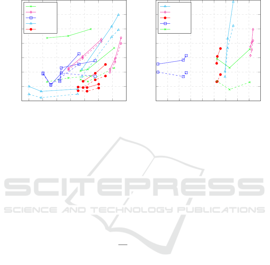
Figure 4: Measured PSNR with different projection methods and sequences:
Left: single-frame prediction (connected points share the same source image), and Right: bidirectional projection.
Dashed curves show the results from mesh-based projection, and solid curves are those from the scale adaptive forward
projection method.
gabean et al., 2010)), image rectification (Ringaby
et al., 2014) and related applications, however we
found that it underperformed in our application and
was therefore omitted. Even Kriging refinement im-
proved the results only marginally. We conclude that
the reason for the omittedly bad performance of Krig-
ing in our application lies in the simple fact that after
the agglomerative clustering too few candidates are
left for Kriging to improve the results significantly.
For image merging, we used W
c
= 0.0000775, W
a
=
0.0375, T
ACmax
= 0.05, and edge suppression. For an
example of how edge suppression performs, see fig-
ure 5 (especially the magenta rectangles).
For downsampling, Gaussian filtering with σ =
π∗S
u
8
(with S
u
the factor by which the original resolution
was upscaled in width and height) worked best.
In figure 4 PSNR of the overall best solution is shown
as a function of coverage (mask area relative to the
image size), to show PSNR as a function of the pro-
jection difficulty.
We also considered frame distance instead, but this
is less correlated with difficulty (correlation of -0.61
compared to 0.68 for coverage), as camera (and ob-
ject) movements can be fast and rapid, or smooth
or even absent. However, coverage does not reflect
changes in texture (due to e.g. lighting) and is thus
not completely accurate. Note that coverage is also
an upper-bound of the portion of the frame that can
be predicted using view prediction.
As can be seen in figure 4 (left) there is a weak
correlation between coverage and PSNR, that grows
stronger for high coverage values. The correlation
would probably have been stronger if other nuisance
parameters, such as illumination and scale change
were controlled for. The correlation is much weaker
for bidirectional projection, see figure 4 (right). This
is explained by blending of projections with different
scale changes.
In table 1, average PSNR and multiscale SSIM (Wang
et al., 2003) values are given for each sequence, for
the different configurations. We concentrated on the
different extensions suggested in this paper, and used
the best configuration for each to show how each of
these perform compared to each other. A compari-
son between with and without Kriging refinement was
omitted, since it performed only barely better and its
effect is therefore nearly unnoticeable.
The multiscale SSIM quality metric was found to per-
form well in a recent study (Ma et al., 2016). It em-
phasizes how well structures are preserved and thus
might give a more accurate view of how well the dif-
ferent methods behave. From an encoder point of
view, PSNR is of more interest, since it is used as
quality metric in nearly all encoders. Thus, the higher
the PSNR value reached by the projection is, the
smaller the residual that needs to be encoded should
be, and the better view projection should perform.
Comparing the results from the bidirectional forward
predictions (both with adaptive and with fixed ker-
nels), especially the mountain1 sequence shows how
much can be gained from using adaptive kernel sizes.
An odd effect in this sequence, is that the bidirec-
tional projections performed on average worse than
the predictions from single images, when fixed splat
Pushing the Limits for View Prediction in Video Coding
73
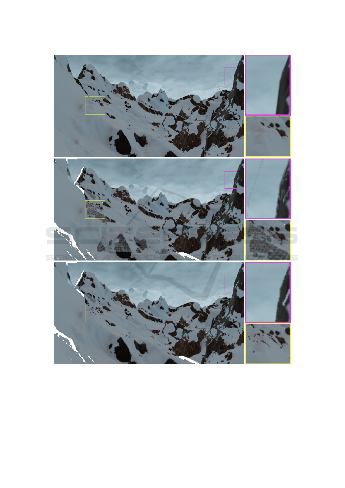
Figure 5: Example of improvements from edge suppression and the scale-adaptive kernel.
Top: Ground-truth frame from the mountain1 sequence with two difficult parts indicated in yellow and magenta. Detail
images of the difficult parts are shown in the right column.
Middle: View projection without edge suppression and the scale-adaptive kernel. Here we can see false edges (e.g. in the
magenta boxes) and foreground objects that are partly covered by a background object (e.g. in the yellow boxes), since the
foreground object had a large scale change and the splatting kernel did not reach all pixels in the projected image. The white
regions, e.g. in the lower left were never seen in the source images are thus impossible to recover.
Bottom: View projection using edge suppresion and scale-adpative kernel, removing most of the artifacts (some artifacts
remain, as the projection was tuned on other sequences).
VISAPP 2017 - International Conference on Computer Vision Theory and Applications
74

Table 1: Average PSNR (top) and multiscale SSIM loss (bottom) values for each sequence using the projection methods
Mesh, Forward, Forward-SA (Forward warp with scale adaptive splatting kernel), Forward-ES (Forward warp with edge
suppression) and Forward-ES-SA (Forward warp with edge suppression and scale adaptive splatting kernel). Multiscale
SSIM loss (i.e. (1 − SSIM)∗ 100) is used to emphasize changes. Best results in each row are shown in bold.
The frames column shows how many frames were used for the predictions (1 for single, 2 for bidirectional).
Note that edge suppression only affects the blended images, thus the results for single frames are identical.
Sequence #frames Mesh Forward Forward-SA Forward-ES Forward-ES-SA
Sleeping 2
1 28.98 29.33 29.38 n/a n/a
2 30.26 31.39 31.44 31.43 31.52
Alley 2
1 27.06 28.30 28.27 n/a n/a
2 30.03 31.77 31.72 31.75 31.83
Temple 2
1 26.50 27.12 27.28 n/a n/a
2 26.77 28.78 28.89 28.56 28.69
Bamboo 1
1 25.12 25.94 25.94 n/a n/a
2 26.00 28.80 28.82 29.22 29.22
Mountain 1
1 26.24 29.85 30.28 n/a n/a
2 25.29 26.96 27.22 24.43 28.88
Sequence #frames Mesh Forward Forward-SA Forward-ES Forward-ES-SA
Sleeping 2
1 3.48 3.61 3.57 n/a n/a
2 2.33 2.15 2.14 2.13 2.07
Alley 2
1 4.96 2.89 2.90 n/a n/a
2 3.26 1.81 1.82 1.81 1.82
Temple 2
1 10.39 9.90 9.76 n/a n/a
2 9.04 7.52 7.44 7.56 7.41
Bamboo 1
1 9.26 9.20 9.19 n/a n/a
2 6.15 4.64 4.62 4.61 4.55
Mountain 1
1 6.82 2.09 2.05 n/a n/a
2 5.73 3.53 3.18 4.62 2.09
kernels were used. Careful examination of the actual
images reveal that some of the scale dependent arti-
facts, that the adaptive splat kernels are supposed to
remove, are still visible (see also figure 5), and thus
these results could be improved further. The reason
for the remaining artifacts are cases where the local
curvatures are very different in perpendicular direc-
tions, and where therefore the outlier removal will
remove the candidates in the direction of the higher
curvature even if these are valid candidates. As the
parameters used are optimized on sequences without
large scale changes, a larger tuning set should be able
to improve the results further, however probably at the
cost that sequences with small scale changes perform
slightly worse.
4 CONCLUSION & FUTURE
WORK
In this paper, we evaluated the performance of dif-
ferent DIBR algorithms, for the application of video
compression. This was done using an exhaustive
search to optimize parameters of a generic forward
warping framework, incorporating the state-of-the-art
methods in this area as well as own contributions.
While we have shown that performance can be
boosted greatly using the right parameters and algo-
rithms, even simple methods such as a mesh-based
warp can generate surprisingly accurate results. How-
ever, mesh-based warp loses more details esepcially
during scale changes, as can be seen in the results on
the mountain1 sequence.
This evaluation was performed on ground-truth data,
to ensure that noise and artifacts are caused by the
DIBR and not by erroneous input data. However, real
RGB+D sensor data may contain noise, reduced depth
resolution (compared to the texture) and artifacts such
as occlusion shadows. Such issues can be dealt with
using depth-map optimization and upsampling, for
which a number of algorithms exist (e.g. (Yang et al.,
2007; Wang et al., 2015; Diebel and Thrun, 2005;
Kopf et al., 2007)) which have been proven to in-
crease accuracy tremendously. Still, an important fu-
ture investigation is to also evaluate performance on
real RGB+D video, where depth has been refined us-
ing one of the above methods.
Pushing the Limits for View Prediction in Video Coding
75

Furthermore, we noticed that effects such as blur and
lighting (e.g. blooming, reflection and shadows, com-
pare also the two pictures on the bottom row in figure
2, especially the false shadow up in the middle) in-
fluence the results significantly. More sophisticated
interpolation methods should give these cases special
consideration, by e.g. explicitly modeling them.
Finally, while PSNR values give a good indication of
how well these methods would work for view predic-
tion, it is an open question how much this will im-
prove coding efficiency in practice. This is especially
true since the projection might lead to deformations or
shifts of the edges, which might be noticeable in the
measured PNSR (and SSIM) values, but which could
easily be corrected by a motion vector.
ACKNOWLEDGEMENT
The research presented in this paper was funded by
Ericsson Research, and in part by the Swedish Re-
search Council, project grant no. 2014-5928.
REFERENCES
Butler, D., Wulff, J., Stanley, G., and Black, M. (2012). A
naturalistic open source movie for optical flow eval-
uation. In Proceedings of European Conference on
Computer Vision, pages 611–625.
Diebel, J. and Thrun, S. (2005). An application of Markov
random fields to range sensing. In In NIPS, pages
291–298. MIT Press.
Dong, J., He, Y., and Ye, Y. (2012). Downsampling filter
for anchor generation for scalable extensions of hevc.
In 99th MPEG meeting.
Iyer, K., Maiti, K., Navathe, B., Kannan, H., and Sharma, A.
(2010). Multiview video coding using depth based 3D
warping. In Proceedings of IEEE International Con-
ference on Multimedia and Expo, pages 1108–1113.
Kopf, J., Cohen, M. F., Lischinski, D., and Uyttendaele, M.
(2007). Joint bilateral upsampling. ACM Transactions
on Graphics, 27(3).
Ma, K., Wu, Q., Wang, Z., Duanmu, Z., Yong, H., Li, H.,
and Zhang, L. (2016). Group mad competition - a
new methodology to compare objective image quality
models. In IEEE Conference on Computer Vision and
Pattern Recognition (CVPR), pages 1664–1673.
Mall, R., Langone, R., and Suykens, J. (2014). Agglom-
erative hierarchical kernel spectral data clustering. In
IEEE Symposium on Computational Intelligence and
Data Mining, pages 9–16.
Mark, W. R., McMillan, L., and Bishop, G. (1997). Post-
rendering 3d warping. In Proceedings of 1997 Sym-
posium on Interactive 3D Graphics, pages 7–16.
Morvan, Y., Farin, D., and de With, P. (2007). Incorpo-
rating depth-image based view-prediction into h.264
for multiview-image coding. In Proceedings of IEEE
International Conference on Image Processing, vol-
ume I, pages 205–208.
Panggabean, M., Tamer, O., and Ronningen, L. (2010).
Parallel image transmission and compression using
windowed kriging interpolation. In IEEE Interna-
tional Symposium on Signal Processing and Informa-
tion Technology, pages 315 – 320.
Ringaby, E., Friman, O., Forss
´
en, P.-E., Opsahl, T.,
Haavardsholm, T., and Ingebjørg K
˚
asen, I. (2014).
Anisotropic scattered data interpolation for pushb-
room image rectification. IEEE Transactions in Image
Processing, 23(5):2302–2314.
Scalzo, M. and Velipasalar, S. (2014). Agglomerative clus-
tering for feature point grouping. In IEEE Interna-
tional Conference on Image Processing (ICIP), pages
4452 – 4456.
Shimizu, S., Sugimoto, and Kojima, A. (2013). Back-
ward view synthesis prediction using virtual depth
map for multiview video plus depth map coding. In Vi-
sual Communications and Image Processing (VCIP),
pages 1–6.
Solh, M. and Regib, G. A. (2010). Hierarchical hole-
filling(HHF): Depth image based rendering without
depth map filtering for 3D-TV. In IEEE International
Workshop on Multimedia and Signal Processing.
Szeliski, R. (2011). Computer Vision: Algorithms and Ap-
plications. Springer Verlag London.
Tian, D., Lai, P.-L., Lopez, P., and Gomila, C. (2009). View
synthesis techniques for 3D video. In Proceedings of
SPIE Applications of Digital Image Processing. SPIE.
Wang, C., Lin, Z., and Chan, S. (2015). Depth map restora-
tion and upsampling for kinect v2 based on ir-depth
consistency and joint adaptive kernel regression. In
IEEE International Symposium onCircuits and Sys-
tems (ISCAS), pages 133–136.
Wang, Z., Simoncelli, E. P., and Bovik, A. C. (2003). Multi-
scale structural similarity for image quality assess-
ment. In 37th IEEE Asilomar Conference on Signals,
Systems and Computers.
Yang, Q., Yang, R., Davis, J., and Nister, D. (2007). Spatial-
depth super resolution for range images. In IEEE Con-
ference on Computer Vision and Pattern Recognition
(CVPR), pages 1–8.
VISAPP 2017 - International Conference on Computer Vision Theory and Applications
76
