
Spatio-temporal Road Detection from Aerial Imagery using CNNs
Bel
´
en Luque, Josep Ramon Morros and Javier Ruiz-Hidalgo
Signal Theory and Communications Department, Universitat Polit
`
ecnica de Catalunya - BarcelonaTech, Barcelona, Spain
luquelopez.belen@gmail.com, {ramon.morros, j.ruiz}@upc.edu
Keywords:
Computer Vision, Road Detection, Segmentation, Drones, Neural Networks, CNNs.
Abstract:
The main goal of this paper is to detect roads from aerial imagery recorded by drones. To achieve this, we
propose a modification of SegNet, a deep fully convolutional neural network for image segmentation. In
order to train this neural network, we have put together a database containing videos of roads from the point
of view of a small commercial drone. Additionally, we have developed an image annotation tool based on
the watershed technique, in order to perform a semi-automatic labeling of the videos in this database. The
experimental results using our modified version of SegNet show a big improvement on the performance of the
neural network when using aerial imagery, obtaining over 90% accuracy.
1 INTRODUCTION
Even though drones were initially developed for mili-
tary purposes, they have become surprisingly popular
for civilian and business use in the past few years. It
is fairly easy to attach a camera to a drone, which al-
lows for a large amount of applications. For instance,
they are used as a support system in firefighting ac-
tivities, as a drone can provide a map of the fire’s
progress without endangering any human life. Drones
are also used for traffic analysis and exploring hard-
to-access areas, where they can provide more mobility
than other technologies. In order to analyze and pro-
cess the images captured by a drone, it is necessary
to use computer vision techniques. However, the na-
ture of these images raises difficulties, as they present
an outdoor location with a complex background. The
camera is in motion, so the background obtained is
not static, but changes from frame to frame. Fur-
thermore, the perspective of a given object can vary
widely depending on the position of the drone in rela-
tion to the ground.
The main goal of this work is detecting a road
from the point of view of a drone, which is necessary -
or very helpful - in a lot of applications, like the ones
mentioned above. The segmentation of the images
is carried out using SegNet (Badrinarayanan et al.,
2015), a deep fully convolutional neural network ar-
chitecture for semantic pixel-wise segmentation, orig-
inally trained to segment an image in 11 classes (sky,
building, pole, road, pavement, tree, sign symbol,
fence, car, pedestrian and bicyclist). However, the
images used for the original training of SegNet are
taken from a car driver’s point of view. This leads
to a poor performance of SegNet when using aerial
imagery, so we have modified and retrained the sys-
tem with a new database and diminished the classes
from 11 to 3 (road, sky and other). We created this
new database by gathering existing videos from dif-
ferent sources. As these videos were unlabelled, we
have also developed a semi-automatic labelling tool
to obtain the necessary ground truth to train a neural
network. Moreover, there is a certain correspondence
between consecutive frames in a video that we use
after the segmentation with SegNet to improve the re-
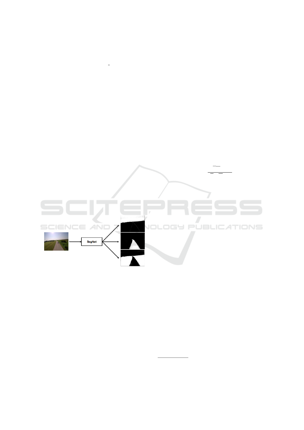
sult, which becomes more consistent and robust. Fig-
ure 1 shows the block diagram of the flow used in this
work.
This paper is organized as follows: In section 2,
we do a brief review of some state-of-the-art tech-
niques for road detection. Next, we explain our
method for doing so in section 3, where we detail both
the image segmentation and the temporal processing
blocks. Afterwards, section 4 describes the creation
and labelling of our new database. Finally, we show
the results we have obtained in section 5, before our
conclusions in the last section.
2 STATE OF THE ART
Getting a computer to recognize a road in an image is
a great challenge. There is a wide variety of surround-
ings where a road can be located. This forces to create
Luque B., Morros J. and Ruiz-Hidalgo J.
Spatio-temporal Road Detection from Aerial Imagery using CNNs.
DOI: 10.5220/0006128904930500
In Proceedings of the 12th International Joint Conference on Computer Vision, Imaging and Computer Graphics Theory and Applications (VISIGRAPP 2017), pages 493-500
ISBN: 978-989-758-225-7
Copyright
c
2017 by SCITEPRESS – Science and Technology Publications, Lda. All rights reserved
493

Figure 1: Block diagram of the developed system.
a quite generic detector in order to obtain good results
in diverse locations, where the colors and illumination
of the road may greatly vary in different scenes. The
first road detectors that were developed focused on
well paved roads with clear edges. In this case, it was
relatively easy to find the limits of the road or even
road marks, using techniques like the Hough trans-
formation (Southall and Taylor, 2001) (Yu and Jain,
1997) or color-based segmentation (Sun et al., 2006)
(Chiu and Lin, 2005) (He et al., 2004). However,
these approaches allow for little variation in the type
of road that can be detected. The Hough transform
will have a poor performance in dirt roads and rural
areas, where it is more likely to find bushes and sand
covering the limit lines and, therefore, complicating
its detection. In turn, the main problem for the color-
based techniques will be the broad diversity of colors
that can present a road depending on the illumination,
material and conditions of the road. Moreover, other
objects with a similar color to the road will be often
found in the scene, giving rise to false positives.
Recently, some more research has been done
in this field, specially to apply it on self-driving
cars. Although good results were obtained with tech-
niques like Support Vector Machines (SVM) (Zhou
et al., 2010) or model-based object detectors (Felzen-
szwalb et al., 2010), a great improvement was made
with the popularization of Convolutional Neural Net-
works (CNN) after the appearance of the AlexNet
(Krizhevsky et al., 2012). Owing to their great perfor-
mance, CNNs are now one of the preferred solutions
for image recognition. One of the recently developed
CNN-based systems is SegNet (Badrinarayanan et al.,
2015), used in this paper.
The vast majority of studies focus on a driver’s
viewpoint, but this approach is very different from
the one we seek in this work, where the images are
captured by a drone with an aerial view of the road.
Although there exist some approaches to road detec-
tion from an aerial viewpoint, they are based on clas-
sical methods such as snakes (Laptev et al., 2000),
histogram based thresholding and lines detection us-
ing the Hough transform (Lin and Saripalli, 2012)
or homography-alignment-based tracking and graph
cuts detection (Zhou et al., 2015). The main con-
tributions of this paper are to extend the current ap-
proaches of road segmentation to aerial imagery us-
ing convolutional neural networks and to provide a
database to do so, as well as a tool for automatically
labeling a video sequence using only the manual seg-
mentation of the first frame.
3 ROAD DETECTION
3.1 Image Segmentation
The first step of the proposed method is to segment
all the frames of a video into different classes, in our
case road, sky and other. To do so, we use SegNet, a
deep convolutional encoder-decoder architecture with
a final pixel-wise classification layer, capable of seg-
menting an image in various classes in real time. This
system achieves state-of-the-art performance and is
trained to recognize road scenes, which makes it a
good starting point for our purpose. However, we
need to slightly modify it to fit our interests better.
One of the parameters to modify is the frequency
of appearance of each class. This is used for class
balancing, which improves the results when the num-
ber of pixels belonging to a class is much lesser than
another (in our case, the classes road and sky are far
less abundant than the class other). The frequency of
appearance is used to weight each class in the neural
network’s error function, so a mistake in the classi-
fication of a pixel belonging to a less frequent class
will be more penalized. As our database and classes
are different from the SegNet original’s, the provided
class frequencies are not coherent with the images
used. In order to compute our own class frequencies,
we use the same equation as the SegNet authors,
α
c
= median f req/ f req(c)
VISAPP 2017 - International Conference on Computer Vision Theory and Applications
494
where freq(c) is the number of pixels in class c di-
vided by the number of pixels that belong to an image
where class c appears, and median freq is the median
of those frequencies.
On another note, as we use a brand new database
that we had to label, we decided to only use 3 classes.
However, in section 5 we will see that we do not train
the neural network from scratch, we fine-tune it in
order to take advantage of the information learned
in its original training. This is done by initializing
the neural network with some pretrained weights and
then training it with the new database. The pretrained
weights we have used are the ones corresponding to
the final model of SegNet. Therefore, the layers of
the network are initially configured to segment an im-
age in 11 classes. In order to deal with the change
on the number of classes, we set the class frequencies
of the remaining 8 classes to 0 in the Softmax layer of
the neural network, where the class balancing is done.
With these changes, SegNet is modified to fit our
purpose. Figure 2 shows the final appearance of the
image segmentation block. SegNet now provides 3
probability images, one for each class. In each of
these images, every pixel is set with its probability
of belonging to the corresponding class. This is done
for all the frames in a video and the resulting proba-
bilities are then passed onto the temporal processing
block.
Figure 2: Input and output of SegNet. The output shows
a probability images for each class (sky, road and other in
this order). The whiter the pixel, the more probable that it
belongs to the corresponding class.
3.2 Temporal Processing
In order to make the most of the temporal character-
istics of the videos, we have added an additional pro-
cessing block after SegNet’s segmentation. We take
advantage of the temporal continuity of the videos,
as they do not have abrupt changes in the scene from
frame to frame. Therefore, we can do an image rec-
tification between a frame and its consecutive with a
minimal error. There exist two main methods to align
two frames. On the one hand, one can look for in-
teresting points (mostly corners) in one of the images
and try to find those same points in the other frame.
Then, the movement of these points from one frame
to the other is calculated, and one of the frames is
transformed to counterbalance the motion of the cam-
era. On the other hand, it is possible to align two
frames taking into account the whole image and not
only some points. This is the method we use, as the
interesting points in our images would mostly belong
to moving vehicles. Therefore, if we took those points
as a reference, we would counterbalance the whole
scene based on the movement of a vehicle, not the
motion of the camera. In order to estimate the trans-
formation that has to be applied to one of the frames
to align them, we use the Enhanced Correlation Co-
efficient (ECC) algorithm (Evangelidis and Psarakis,
2008). This iterative algorithm provides the transfor-
mation that maximizes the correlation coefficient (1)
between the first frame (i
r
) and the second one after it
is transformed (i
w
) with transformation parameters p.
ρ(p) =
i
t
r
i
w
(p)
ki
r
kki
w
(p)k
(1)
Once we have found the optimum transformation
we can align both frames and, therefore, know which
pixel on the first frame corresponds to one on the sec-
ond frame (although some of them will remain un-
paired). With this, we can add the probabilities of
a pixel throughout a sequence of images in a video,
thus obtaining a cumulative probability for each class.
When classifying a pixel of a frame, we will choose
the class with the highest cumulative probability, tak-
ing into account the last 10 frames. The results ob-
tained with this additional processing are more robust
and coherent in time. The detail on the results can be
found in section 5.
4 DATABASE
Due to the main component of our road detector be-
ing a neural network, we need to carry out a training
phase prior to obtaining a good performance. How-
ever, the training of a neural network requires a la-
belled database. As we could not find a suitable one
for our work nor had the resources to create enough
material of our own, we gathered unlabelled videos
from different sources and labelled them ourselves.
This database
1
consists of 3.323 images from 22 dif-
ferent scenes. All the images have been captured by
a flying drone and the main element in the scene is a
road, but the illumination and viewpoint varies greatly
1
https://imatge.upc.edu/web/resources/spatio-temporal-
road-detection-aerial-imagery-using-cnns-dataset
Spatio-temporal Road Detection from Aerial Imagery using CNNs
495
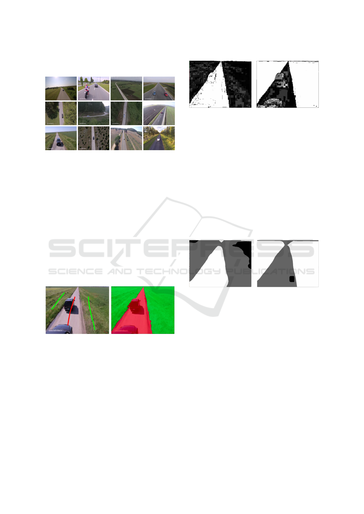
in each video (Figure 3). The surroundings are also
varied, although most of them are rural.
Figure 3: Some examples of images in the drones’ database.
In order not to manually label thousands of im-
ages, we also developed a semi-automatic labelling
tool
1
for this purpose, using classical methods instead
of deep learning. With this tool it is only necessary
to manually label the first frame of each video, and
the algorithm will adequately propagate these labels
to the rest of the sequence. If there was an abrupt
change in a scene, a frame in the middle of the video
sequence can also be manually labelled in order to re-
sume the propagation to the rest of the sequence tak-
ing those labels as the initial point. The steps of the
developed algorithm are the following:
1. Manually define a marker for each desired region
(road, sky and other in our case) on the first frame
of a video and apply the watershed algorithm to
obtain a segmented image (Figure 4).
Figure 4: On the left, the first frame of a video sequence,
where some seeds or markers have been defined for the road
(red) and other (green) classes. On the right, the segmented
image using the watershed technique with the defined mark-
ers.
2. Calculate the histogram for each region. Prior to
doing so, we convert the RGB image to the HSV
color space and keep only the first channel (Hue).
3. Do a back projection of the histograms. For every
pixel in the image, we determine its probability
of belonging to a class by finding the value for
its color in the histogram, which we previously
normalize (Figure 5).
Figure 5: Back projection of the class road (left) and other
(right). They show the probability of each pixel on the im-
age to belong to the corresponding class. The whiter the
pixel, the more probable that it belongs to the class.
4. Apply thresholds and a median filter. We adapt
the obtained probabilities to watershed markers,
dividing them in three groups:
• If probability = 0: the pixel does not belong to
a given class.
• If 0 < probability < 0.8: undefined, it will not
count as a marker.
• If probability > 0.8: the pixel sure belongs to a
given class and will be used as a marker on the
next frame.
A median filter is also applied, to homogenize the
regions of each class. (Figure 6).
Figure 6: Resulting zones after converting the probabili-
ties to markers and homogenizing the regions. For each
class, road on the left and other on the right, there is a
safe zone where the pixels sure belong to the correspond-
ing class (white), a fuzzy zone where no markers will be
defined (gray) and an unsafe zone that indicates the pixels
that do not belong to the class (black).
5. Eliminate the markers on the edges. The lim-
its among watershed regions can be located and
dilated, creating a fuzzy zone between regions,
where no watershed marker will be set. This way,
the contour of the regions in an image will be de-
termined by the watershed algorithm, instead of
the markers of the previous frame.
6. Eliminate conflicting markers. A marker for a
given class can only be located in an area that be-
longed to that same class in the previous frame.
Thus, a region will only expand to adjacent zones
and sporadic markers will be avoided. As a coun-
terpoint, new elements in an image won’t be de-
tected if they are not in contact with a labelled
VISAPP 2017 - International Conference on Computer Vision Theory and Applications
496
element of the same class. However, this is not
often a big issue in the kind of videos used for
this paper, as there are no abrupt changes in the
scenes. In any case, a mid-sequence frame can
also be manually labelled according to the desired
regions and propagate the labels from that point in
the video.
7. Apply the watershed algorithm in the next frame
using the defined markers and go back to step 2
(Figure 7).
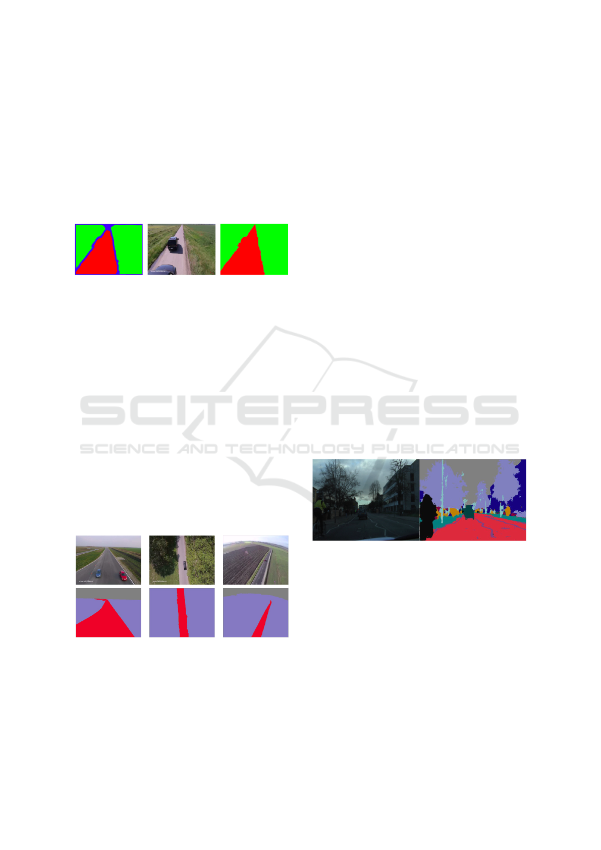
Figure 7: On the left, the resulting markers where red be-
longs to the class road, green belongs to the class other and
blue determines the undefined regions. On the right, the
segmented image after applying the watershed technique on
the second frame (image on the center) using the markers
obtained.
Some examples of the segmentation obtained with the
developed system are shown in Figure 8. We can only
do a subjective evaluation of these results, as we do
not have any ground truth to compare the results with.
In fact, this segmentation will be used as the ground
truth from now on. As for the developed method, the
results are fairly good and it has a fast execution time,
almost in real time. Even though the labels of the first
frame have to be manually defined, this also gives the
user a chance to define the desired classes. As a coun-
terpoint, if the markers of a certain region disappear at
any moment, it will not be possible to automatically
recover them. However, the process can be stopped
and then resumed taking any frame of the video as
the initial point, with a redefinition of the markers.
Figure 8: In the first row, some images of the drones’
database. In the second row, their corresponding labels ob-
tained with the developed labelling tool.
Once the database is labelled, we can train the
neural network. In order to prevent overfitting, the
database is divided in three sets: train, validation and
test. The first one is used to train the neural network
and then the results are evaluated with the validation
set. Finally, the neural network is evaluated with the
test set to check that it delivers a good performance
for images that were not used in the training process.
If the neural network is not overfitted, the results ob-
tained with the three sets should be similar. The de-
tails on the trainings we carried out can be found in
the next section.
5 EXPERIMENTAL RESULTS
5.1 Image Segmentation
In order to evaluate the results obtained with the dif-
ferent trainings of SegNet we use the same method
as the authors of this architecture, calculating the per-
centage of well classified pixels in each image. The
set of images for the test consists of 1.199 frames of
several videos recorded by drones.
The SegNet was initially trained for segmenting
images captured from a driver’s point of view. For
that reason, it does not recognize the different objects
in our set of images, as the viewpoint is very differ-
ent. In Figure 9 there is an example of the segmenta-
tion obtained when using the original SegNet in im-
ages of the database that was used for its training, the
CamVid data set. The segmentation of these images
is very good and takes into account SegNet’s original
11 classes.
Figure 9: Image of the CamVid database, segmented with
the original SegNet.
If we use the same original configuration of Seg-
Net to classify images of the database used in this pa-
per, the results are considerably worse. In Figure 10
we can see how some plants and trees are classified as
trees (sky blue), but the rest of the classes are not cor-
rectly detected. Even if we regrouped the 11 classes in
only 3 (sky, road and others), the classification would
still be terrible.
Given these bad results, we proceeded to retrain
the our modified version of SegNet with the database
detailed in section 4. The first experiment was to train
the SegNet from scratch. We trained two versions
with this database, one with class balancing and one
Spatio-temporal Road Detection from Aerial Imagery using CNNs
497
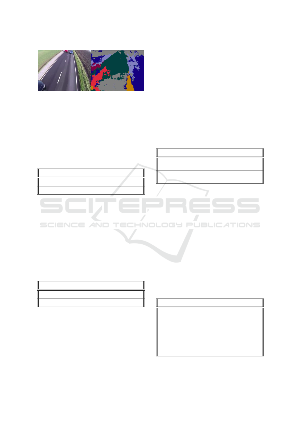
Figure 10: Image on the drones’ database, segmented with
the original SegNet. Gray belongs to the sky, green to vehi-
cles, yellow to pedestrians, dark blue to buildings, sky blue
to trees, maroon to road and red to pavement.
without. The results in Table 1 indicate that the train-
ing without class balancing provides better global re-
sults. However, the sky and road are better classi-
fied when we use class balancing, as they are minority
classes that benefit from class balancing.
Table 1: Evaluation of SegNet trained from scratch with this
paper’s database.
Precision (%)
Sky Road Other Global
No class balancing
76.59 70.61 95.03 85.60
Class balancing
77.71 71.54 91.07 83.80
These results are clearly improvable so, in order to
take advantage of the information generated in Seg-
Net’s original training - which provides very good
results as seen in Figure 9 -, we fine-tuned our neu-
ral network instead of retraining it from scratch. We
used SegNet’s final model, trained with 3.5K images
as mentioned in the previous section, and fine-tuned it
with the drones’ database. The results of this training
are in Table 2, and show a big improvement in relation
to training the neural network from scratch.
Table 2: Evaluation of the original SegNet fine-tuned
with this paper’s database, without the temporal processing
block.
Precision (%)
Sky Road Other Global
No class balancing
99.48 84.52 95.06 91.82
Class balancing
99.70 93.18 91.53 93.13
In the projects that deal with images is equally,
if not more, important to evaluate the results sub-
jectively than objectively. In Figure 11 we can see
a big improvement in contour definition when fine-
tuning instead of training from scratch. Moreover, we
can observe how including class balancing provides
more homogeneous classes, as some random groups
of badly classified pixels disappear.
5.2 Temporal Processing
When adding a temporal processing block after Seg-
Net’s pixel-wise classification, isolated badly classi-
fied pixels are corrected. The classes become more
homogeneous and the classification is more robust
over time. In order to decide the number of frames
to take into account and the maximum iterations of
the ECC algorithm, we perform several tests, using
our fine-tuned version of SegNet, with class balanc-
ing. Table 3 shows the results obtained when vary-
ing the maximum number of iterations allowed on the
ECC iterative algorithm.
Table 3: Evaluation of the temporal processing block’s per-
formance depending on the number of maximum iterations
allowed on the ECC iterative algorithm.
Precision (%)
Sky Road Other Global
10 frames
5 iterations
99.62 94.21 92.45 93.98
10 frames
100 iterations
99.62 94.24 92.44 93.97
Both objective and subjective results are almost
identical for 5 or 100 iterations in the ECC algo-
rithm, but the latest causes a big delay in the execu-
tion time of the system. Thus, as the results are very
similar but one of the options is considerably faster
than the other, we set 5 as the maximum iterations
allowed in the ECC algorithm for image alignment.
With the iterations set to 5, we modify the number of
past frames to take into account when processing the
current frame. The best result, both objectively and
subjectively, is obtained when taking into account the
last 10 frames (Table 4) and using 5 iterations for the
ECC algorithm, which is our final configuration of the
system.
Table 4: Evaluation of the temporal processing block’s per-
formance depending on the number of past frames taken
into account. For each evaluation, the precision and recall
values are provided, in %.
Precision/Recall
Sky Road Other Global
5 frames,
98.97 92.56 89.90 91.31
5 iterations
85.60 88.44 95.51 89.85
10 frames,
99.62 94.24 92.44 93.97
5 iterations
90.78 91.11 97.06 92.98
15 frames,
98.42 75.28 91.62 92.35
5 iterations
89.77 91.01 95.14 91.97
VISAPP 2017 - International Conference on Computer Vision Theory and Applications
498
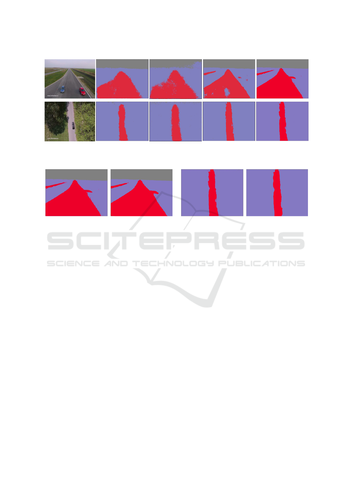
Figure 11: Comparison of the results obtained with different trainings of SegNet. In the first column, the input image. In the
second and third column, the result obtained after training SegNet from scratch, without and with class balancing. In the last
two columns, the result obtained after fine-tuning SegNet, without and with class balancing.
Figure 12: Comparison of the segmentation obtained with SegNet and the one obtained after the temporal processing.
The modification of these parameters do not cause
a huge difference, so we have omitted the visual re-
sults of each of the tests. However, Figure 12 presents
the comparison between the result obtained at the end
of the neural network and the one obtained after the
temporal processing, although the improvement is not
as notable in a few images as in a video sequence.
6 CONCLUSIONS
Applying computer vision on drones is a very new and
extensive field that will give raise to many new devel-
opments in the following years. In turn, road detec-
tion will play an important role in these applications,
as drones are mostly used in outside locations, where
roads are almost always present. Therefore, in the
vast majority of new developments involving drones,
roads will probably be either the object of study or
used as a reference for location.
Defining a generic road and vehicle detector is
complex, specially due to the big variety of input im-
ages. If it was defined that the imagery would al-
ways be captured from the same point of view or that
the conditions of the road and surroundings would al-
ways be similar, the adjustment of some parameters in
the detector would enhance the results. However, the
challenge of this paper was to develop a very generic
detector that would work in very diverse surround-
ings.
In this work, we extend the most popular approach
to road detection, which is working on images from a
driver’s viewpoint, to aerial imagery. We prove with
our experimental results that it is possible to detect
a road from very diverse aerial points of view with
deep learning methods, obtaining an accuracy of over
90%. Moreover, we provide a labelled database of
aerial video sequences where roads are the main ob-
ject of interest, as well as the semi-automatic tool we
have developed to label it.
ACKNOWLEDGEMENT
This work has been developed in the framework of
projects TEC2013-43935-R and TEC2016-75976-R,
financed by the Spanish Ministerio de Economia y
Competitividad and the European Regional Develop-
ment Fund (ERDF).
REFERENCES
Badrinarayanan, V., Kendall, A., and Cipolla, R. (2015).
SegNet: A Deep Convolutional Encoder-Decoder
Spatio-temporal Road Detection from Aerial Imagery using CNNs
499

Architecture for Image Segmentation. CoRR,
abs/1511.0.
Chiu, K.-Y. and Lin, S.-F. (2005). Lane detection using
color-based segmentation. pages 706–711.
Evangelidis, G. D. and Psarakis, E. Z. (2008). Paramet-
ric image alignment using enhanced correlation co-
efficient maximization. IEEE Transactions on Pat-
tern Analysis and Machine Intelligence, 30(10):1858–
1865.
Felzenszwalb, P., Girshick, R., McAllester, D., and Ra-
manan, D. (2010). Object detection with discrimina-
tively trained part based models. IEEE Trans. Pattern
Analysis and Machine Intelligence, 32(9):1627–1645.
He, Y., Wang, H., and Zhang, B. (2004). Color-based road
detection in urban traffic scenes. IEEE Transactions
on Intelligent Transportation Systems, 5(4):309–318.
Krizhevsky, A., Sutskever, I., and Hinton, G. (2012). Im-
agenet classification with deep convolutional neural
networks. Proceedings of Neural Information and
Processing Systems.
Laptev, I., Mayer, H., Lindeberg, T., Eckstein, W., Steger,
C., and Baumgartner, A. (2000). Automatic extraction
of roads from aerial images based on scale space and
snakes. Machine Vision and Applications, 12(1):23–
31.
Lin, Y. and Saripalli, S. (2012). Road detection from aerial
imagery. In 2012 IEEE International Conference on
Robotics and Automation, pages 3588–3593.
Southall, B. and Taylor, C. J. (2001). Stochastic road shape
estimation. pages 205–212.
Sun, T.-Y., Tsai, S.-J., and Chan, V. (2006). Hsi color model
based lane-marking detection. pages 1168–1172.
Yu, B. and Jain, A. K. (1997). Lane boundary detection
using a multiresolution hough transform. volume 2,
pages 748–751.
Zhou, H., Kong, H., Wei, L., Creighton, D., and Nahavandi,
S. (2015). Efficient road detection and tracking for
unmanned aerial vehicle. IEEE Transactions on Intel-
ligent Transportation Systems, 16(1):297–309.
Zhou, S., Gong, J., Xiong, G., Chen, H., and Iagnemma,
K. (2010). Road detection using support vector ma-
chine based on online learning and evaluation. IEEE
Intelligent Vehicles Symposium, pages 256–261.
VISAPP 2017 - International Conference on Computer Vision Theory and Applications
500
