
Pattern Width Description through Disk Cover
Application to Digital Font Recognition
Nikita Lomov and Leonid Mestetskiy
Moscow State University, Faculty of Computational Mathematics and Cybernetics, Moscow, Russia
{nikita-lomov, mestlm}@mail.ru
Keywords: Disk Cover, Morphological Width, Polygonal Figure, Medial Representation, Skeleton, Radial Function,
Bicircle, Font Comparing.
Abstract: We consider the concept of "the width of a figure" for objects of complex shapes in order to use it as an
integral morphological descriptor in image recognition tasks. In this article we propose a new approach to
the description of this concept on the basis of the figures covering by disks of a certain size. The area of the
disk cover as a function of the covering disc size is a shape descriptor. Original method for analytical
calculation the area of disk cover of polygonal shapes is presented. The method is universal because there is
always the possibility of polygonal approximating of complex digital binary images and geometric objects
with nonlinear boundary. The method is based on the medial representation of the polygonal figure as a
skeleton and a radial function. Our approach ensures high accuracy and computational efficiency calculate
the area of disk cover. The effectiveness of the proposed approach is demonstrated for applications in
computer font’s recognition problem.
1 INTRODUCTION
The width of the objects is an important feature of
image shape. This feature cannot be well described
by a scalar value, such as "average" width, for the
objects of complex shape, in which the different
parts have different width and length. Therefore, the
description of width “distribution” that characterizes
the whole range of its values is required to be used
as width descriptor.
Local description of the width can be based on
the size of the primitive, which can be inscribed in
the object. The larger width of the object, the larger
the size of the primitive. If we inscribe in the object
the primitives of a given size, such as disks of a
certain diameter, the part of the object covered by
the primitives can be considered as a region of a
given width. Then the function describing the
dependence of the region area from the primitive
size can be regarded as an integral description of the
object width. This article proposes an approach to
the construction of the image width descriptor,
which is based on the area of the disk cover of the
object (Fig.1). Selecting a disk as primitive provides
invariance of the descriptor to the shift, rotation and
scaling of images.
The object width descriptor is a diagram
representing the dependency of the cover area from
the size of covering disks (Fig.2).
Figure 1: Disk covers of the “lizard” figure (on the right
the examples of covering disks are shown).
484
Lomov N. and Mestetskiy L.
Pattern Width Description through Disk Cover - Application to Digital Font Recognition.
DOI: 10.5220/0006128804840492
In Proceedings of the 12th International Joint Conference on Computer Vision, Imaging and Computer Graphics Theory and Applications (VISIGRAPP 2017), pages 484-492
ISBN: 978-989-758-225-7
Copyright
c
2017 by SCITEPRESS – Science and Technology Publications, Lda. All rights reserved
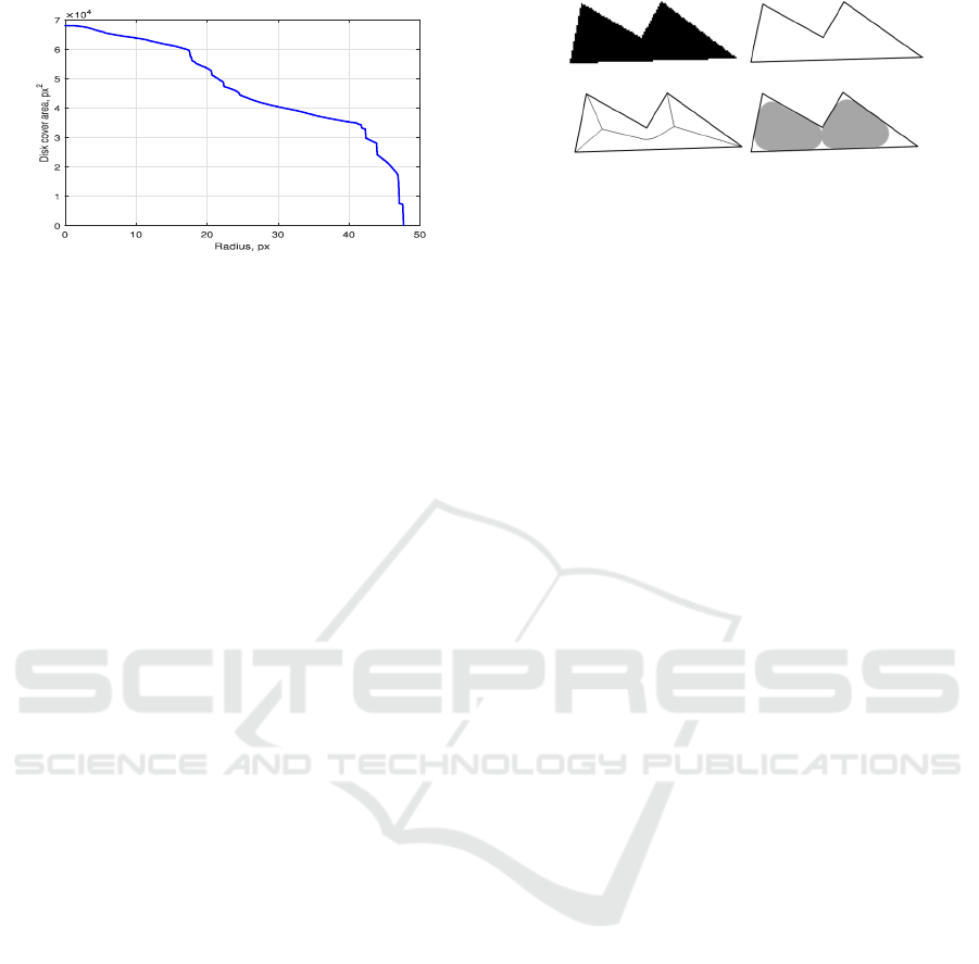
Figure 2: Diagram of the dependency of disk cover area of
the “lizard” figure from the size (radius) of covering disks.
To compute the cover area, the method of pattern
spectrum (Maragos, 1989), based on a discrete
mathematical morphology (Serra, 1982), can be
applied. In this case, the object width descriptor is
the pattern spectrum diagram, constructed on the
base of morphological opening operation using a
disc structuring element. An example of this
approach is described in (Ramirez-Cortes et al.,
2008). Pattern spectrum method allows a simple
software implementation, however, it has a high
computational complexity, especially when working
with large high-resolution images. To cope with this
problem in (Vizilter and Sidyakin, 2012, 2014) a
combined discrete-continuous approach to the
calculation of the pattern spectrum was proposed,
which allowed significantly reduce the computation
time, but not so much. The task cannot be solved in
real-time of the computer vision systems.
Our approach is aimed at drastically reducing the
computation time of the cover area through the use
of a continuous model of an image shape.
Continuous model is a polygonal shape
approximating a digital image. Selecting a polygonal
shape (a polygon with polygonal holes) as a model
of the object shape is due to two reasons. On the one
hand, polygonal shapes can accurately approximate
the boundary of complex objects represented by
discrete raster images. On the other hand, for the
polygonal figure the regions of a given width can be
described using the medial representation – the
skeleton and the radial function. A medial
representation of a polygonal shape can be obtained
with high-performance computational geometry
algorithms (Mestetskiy, 2008).
(a) (b)
(c) (d)
Figure 3: Continuous model of the disk cover for binary
image: a) binary image, b) approximating polygonal figure
c) its skeleton, d) example of r-cover.
Our method of the calculation of the disk cover
area for objects on bitmap images includes the
following steps:
1. Approximation of a binary image by a
polygonal shape.
2. Medial representation of a polygonal shape in
the form of the skeleton and the radial
function based on Voronoi diagrams of line
segments that constitute the shape boundary.
3. Representation of a complex-shaped
polygonal figure as a union of bicircles –
elementary geometric shapes corresponding
to the edges of the skeleton.
4. Representation of the figure disk cover as the
union of a subset of bicircles and calculating
the cover area through bicircles' areas.
5. Construction of the distribution function of
the disk cover area as a function of the disk
size.
2 DISK COVER AND FIGURE
SKELETON
Definition 1. A figure is a closed region in the plane
bounded by a finite number of disjoint closed Jordan
curves.
Definition 2. A circle is considered to be empty
if it is located entirely in the figure.
Definition 3. Disk -cover of the figure is the
union of all empty circles of the radius . Examples
of disk -cover for different values of are shown in
Fig.1.
Definition 4. -area of the figure is the area of its
disk -cover.
According to this definition, the area of the entire
figure is its 0-area.
Definition 5. Morphological width of the
figure is its -area as a function of . Morphological
width is a non-increasing function of the .
Morphological width could be calculated by
using pattern spectrum (Maragos, 1989) through the
Pattern Width Description through Disk Cover - Application to Digital Font Recognition
485

opening operation of a discrete mathematical
morphology (Serra, 1982). The disk is used as a
primitive. This approach requires a lot of
computation time, and may be applied only to
discrete images. Our method is much faster and is
more universal because it allows you to work with
discrete and continuous images through
approximation by polygonal figure.
Definition 6. An inscribed circle of the figure is
an empty circle, which is the maximum, i.e., is not
contained in any other empty circle.
Definition 7. A skeleton of a figure is the set of
all points that are centers of inscribed circles.
Definition 8. The radial function is defined in
the skeleton points and assigns to the skeleton point
the radius of the inscribed circle centered at this
point.
Obviously, each empty circle of radius more than
can be represented as the union of empty circles of
radius . Therefore, any inscribed circle with radius
or more is contained in the disk -cover.
Consequently, the disk -cover of the figure
coincides with the union of all the inscribed circles
of radius at least . The centers of the inscribed
circles constitute a subset of the skeleton points.
Thus, for calculating the morphological width of the
figure it is sufficient to consider only the circles
whose centers lie on the skeleton. The challenge is
to obtain for given values of argument the
corresponding values of figure -area. The solution
to this problem for the polygonal shapes will be
obtained in an explicit form.
3 POLYGONAL FIGURES AND
BICIRCLES
Definition 9. A polygonal figure is a figure whose
boundary consists of closed polylines.
The boundary of a polygonal figure can be
represented as the union of a finite number of
subsets, called sites: point-sites (vertices of the
figure) and segment-sites (sides of the figure without
end points).
A skeleton of a polygonal figure (Fig.4) looks
like geometric graph whose edges are segments of
straight lines and quadratic parabolas, and the
vertices are the endpoints of edges. Each edge is a
connected set of points that are centers of inscribed
circles having the same incident pair of sites, called
site-generators of the edge. If both site-generators
are of the same type (two point-sites or two
segment-sites) then the edge is a straight line
segment. If site-generators are of different types
(point-site and segment-site) then the edge is a
segment of a quadratic parabola.
Figure 4: Polygonal figure and its skeleton.
Polygonal approximation of the digital binary
image and the construction of the continuous
skeleton and radial function are performed by
means of high-performance algorithms
(Mestetskiy, 2008). The proposed method for
calculating -area, using the special properties of a
skeleton of a polygonal shape, is based on the
decomposition of the figure on the constituent
elements – bicircles.
Definition 10. A bicircle is the union of all
inscribed circles centered on one edge of the
skeleton. The edge line is called the axis of the
bicircle.
Three types of bicircles are distinguished
depending on the pair of their site-generators: linear
(two segment-sites – Fig.5a-b), parabolic (segment-
site and point-site – Fig.5c) and hyperbolic (two
point-sites – Fig.5d). This terminology is caused by
the dependency of the radial function on the position
of a point on the axis of the bicircle.
Circles with centers at the vertices of the
skeleton are called the end circles of the bicircle.
The boundary of the bicircle is the envelope of the
family of its constituent circles. The boundaries of
linear and parabolic bicircles include, fully or
partially, their generating segment-sites (Fig.5a-c).
In addition, the boundaries of all kind of bicircles
contain arcs of end circles.
(a) (b) (c) (d)
Figure 5: Bicircles: axes, proper regions, external sectors
of end circles.
Definition 11. The sector of end circle relied on
the arc of the bicircle boundary is called an external
sector of a bicircle.
VISAPP 2017 - International Conference on Computer Vision Theory and Applications
486

Definition 12. A spoke is a line segment
connecting the skeleton point with the nearest point
of figure boundary.
Definition 13. A proper region of a bicycle is the
union of all spokes of the bicircle incident to points
of its axis.
The bicircle is the union of its proper region and
the pair of external sectors. The shape of the proper
area depends on the type of bicircle (Fig.5). For a
linear bicycle it is the union of two triangles (Fig.5a)
or two trapezoids (Fig.5b). In the parabolic bicircle
it is a “house-shaped” figure, which can be regarded
as the union of a trapezoid and a triangle (Fig.5c), in
the hyperbolic one it is the union of two triangles
(Fig.5d).
Figure 6: Coverage of the polygonal figure by proper
regions of bicircles.
Let is a polygonal figure,
is a subset of the
figure formed by the union of all spokes of length
and more. It is obvious that
is entirely contained
in -cover. Proper areas of bicircles form the cover
of the whole polygonal figure, the cover coincides
with the union of all spokes, i.e.
(Fig.6).
Definition 14. Bicircle is called monotonic if the
radial function monotonically decreases or increases
along its axis.
It is clear that a linear bicircle is monotonic,
because the linear radial function is monotonic on
the axis. A linear bicircle of constant width
considered to be monotonic by definition.
In the parabolic bicircle, if the vertex of the
parabola is an interior point of the bicircle axis,
when passing through the vertex the behavior of the
radial function changes from the decreasing to the
increasing (Fig.5c). The vertex of the parabola is a
point of local minimum of the radial function and
the bicycle at this time is not monotonic. In other
cases, when the vertex of the parabola lies outside
the axis or coincides with the end point of the axis,
the parabolic bicircle is monotonic.
In the hyperbolic bicircle, the monotonic
property is determined by the position of the centers
of end circles with respect to the site line (the line
passing through the point-sites). If the centers are on
different sides of this line, the point of intersection
of this line with the bicircle axis is inside the axis
and the minimum of radial function is achieved in
this point – therefore, the bicircle is not monotonic
(Fig. 5d). In other cases, the hyperbolic bicircle is
monotonic.
Calculation of morphological width for
monotonic bicircles involves a simpler problem than
for non-monotonic ones. Therefore each non-
monotonic bicircle can be replaced with a pair of
monotonic ones. So its axis can be divided into two
monotonic segments by adding vertices in the
bicircles’ minimal points and splitting the respective
edges into two parts. In the example (Fig.6) four
extreme bicircles are divided into monotonic pairs.
The dotted line shows the corresponding proper
areas of the bicircles.
4 PROPER REGIONS AND
EXTERNAL SECTORS
Figure 6 presents the monotonic bicircles of all three
types. Here, and are the radii of the small and
the large end circles, is the distance between their
centers. If the bicircle is linear or parabolic, it has
the generating segment-site, and then is the length
of the projection of the bicycle axis at this site:
.
In the parabolic bicircle is the distance between
the point-site and a line of the segment-site (the
focal parameter of the parabola). In the hyperbolic
bicircle is the distance between point-sites.
For the linear bicircle (Fig.7a) the proper region
area is determined as the sum of the areas of two
trapezoids, with the bases and and the height :
2∙
∙
∙.
(1)
The angular size of the external sector of the
small end circle is
22∙
.
(2)
For parabolic bicircle (Fig.7b) the proper region
area is composed of the area of the same trapezoid
and the area of the triangle with vertices at the
centers of end circles and at the point-site. The area
of the triangle is calculated by Heron's formula:
∙
, (3)
where /2.
The angular size of the external sector of the
small end circle of parabolic bicircle is
.
(4)
Pattern Width Description through Disk Cover - Application to Digital Font Recognition
487
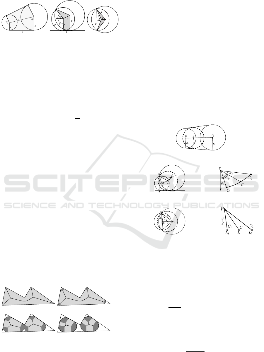
(a) (b) (c)
Figure 7: Proper regions and external sectors of bicircles:
(a) linear, (b) parabolic, (c) hyperbolic.
Proper region area of the hyperbolic bicircle
(Fig.7c) is the sum of the areas of the two triangles,
calculated according to Heron's formula:
2
.
(5)
The angular size of the external sector of the
small end circle is
2
.
(6)
5 TRUNCATED BICIRCLES
Disk -cover of the polygonal figure at 0
coincides with the polygonal figure. As increases,
the cover shrinks and the part of the figure, covered
with disks, diminishes (Fig.8). This cover is a figure
whose boundary consists of line segments and arcs.
Disk -cover is the union of circles with a radius
greater than or equal to , inscribed in the polygonal
figure. We call the set of the centers of these circles
the axis of the -cover. Obviously, the axis of the -
cover is the subset of the polygonal figure skeleton.
This subset is connected at small values of , but as
increses it can split into several connected
components (Fig.8).
Therefore, the polygonal figure skeleton is
divided into two parts: -cover axis – the subset
where the radial function is equal to or more, and
the rest – the subset where the radial function is less
than . Both of these subsets can be considered as
geometric graphs.
(a) (b)
(c) (d)
Figure 8: Changing of disk -cover with increasing disk
radius.
For 0, all bicircles of the polygonal figure
are broken down into three groups: wide (all the
circles of the bicircle belongs to the -cover
completely), narrow (no circle belongs completely),
and truncated (part of the circles belong completely).
Let
and
are the minimum and the
maximum radii of circles in the monotonic bicircle.
Than
in the wide bicircle, and
in the
narrow bicircle.
If
, then the -cover includes only
those circles of the bicircle, whose radius is not less
than . We define the truncation operation of such
bicircle, which is to remove the circles with a radius
smaller than . The resulting new bicircle will be
called truncated. The minimum circle of the
truncated bicycle changes to the circle of radius r,
and the maximum one remains the circle with a
radius
.
(a)
(b)
(c)
Figure 9: Correction of truncated bicircles.
Let
,
are the centers of the small and the
great end circles. We determine the new position of
the small end circle. Let the point is the desired
center of the circle with radius (Fig.9).
For the linear bicircle (Fig.9a), we have
∙,
where
. In the particular case when
, we suppose 0.
For the parabolic bicircle (Fig.9b) choose a polar
coordinate system , with the origin at the point-
site of the bicircle and the axis orthogonal to the
segment-site. The equation of the parabola in these
coordinates is
, where is the focal
parameter of the parabola. The end circles centers
VISAPP 2017 - International Conference on Computer Vision Theory and Applications
488

have coordinates
,
and
,
, where
1,
1. The
required point is ,,
1
Without loss of generality, we assume
.
Vector
is obtained through rotating
by angle
and multiplying by factor
. Then the
desired center of the circle is
∙∙
,
where is the rotation matrix by angle :
cos sin
sin cos
.
In the hyperbolic bicircle (Fig.9c) the point
lies between
and
. Let q is the distance between
point-sites. If is a point-site, the projections of the
vectors
,
,
on the bicircle axis have
lengths
|
|
,
|
|
,
|
|
.
Then
∙, where
.
These formulas allow us to find a new position
of the small end circle, then the calculation of the
area of the bicircle and the angular sizes of the
external sectors is carried out by the same formulas
(1)‒(6), as for wide bicircles.
Therefore, the disk -cover is the union of two
sets of bicircles: full bicircles, where
, and
truncated bicircles, where
. This
cover is composed from proper regions of these
bicircles and external sectors of small circles of the
truncated bicircles.
At Figure 8 proper regions are highlighted in
light gray, and the external sectors – in dark gray.
The total area of the union of the proper regions is
the sum of areas of bicircles’ proper regions.
End circles of truncated bicircles in the -cover
have a radius . The area of the external sector with
an angle is
∙
. But the sectors can have
a nontrivial intersection (Fig.8c).
6 BICIRCLES' INTERSECTIONS
Define those of the bicircles, which can have
significant intersections with each other. When
calculating -area it is only necessary to find the
intersections of adjacent bicircles, i.e. those between
which gaps are formed by removing narrow bicircles
having a width smaller than .
We are interested in only the external sectors of
the small end circles of the bicircles. In the
monotonic bicircle the angular size of the external
sectors of the small end circle .
Definition 15. Two truncated bicircles in the -
cover called adjacent if there is a route in the
skeleton connecting the centers of the end circles,
such that the radial function at all points of the route
is less than .
The external sector of the truncated bicircle may
have the intersection not only with the external
sector of another bicycle, but also with its proper
region. Figure 9 shows examples of possible mutual
arrangements of the external sectors of the two
truncated bicircles. In the first case (Fig.10a) in the
intersection of two sectors the “lens” figure, the
boundary of which consists of two equal circular
arcs, is formed. In the second case (Fig.10b) the
intersection of the sectors is a more complex figure
whose boundary includes straight-line segments of
the spokes and the circular arcs. The gray
highlighted areas in Figure 10 are formed by the
union of the external sectors except for the
intersection of them with the proper areas of the
bicircles. Such areas will be called the outer zone of
the bicircle pair.
(a) (b)
Figure 10: Mutual arrangement of the pair of crossing
external sectors of truncated bicircles.
We denote:
is the area of the end circles of the
bicircles;
is the area of the lens formed by the
intersection of the end circles;
,
are the areas of the bicircles’
external sectors;
,
are the areas of internal sectors of
the end circles.
Internal sector is the addition of the external
sector in the end circle. Internal sectors of two
adjacent truncated bicircles do not intersect each
other. Since the angular size of the external sector
does not exceed , it turns out that the internal sector
size is not less than .
The area of the outer zone formed by a pair of
external sectors of the two intersecting truncated
Pattern Width Description through Disk Cover - Application to Digital Font Recognition
489

bicircles is the sum of the areas of these sectors less
the area of the lens formed by the intersection of the
end circles:
.
(7)
Indeed, the total area of the union of two
intersecting end circles is equal to
2
.
Since internal sectors of the circles do not
intersect:
2
.
Obviously,
.
Taking this into account, we obtain the desired
relation to the area of the outer zone:
.
Let
,
are the angular sizes of two
intersecting external sectors. Then
∙
,
∙
.
The angular size of the lens formed by the two
circles of radius , with centers located at a distance
2 of each other, is
.
The area of this lens is
sin
.
Thus, the area (7) of the outer zone of the pair of
intersecting bicircles is equal to
∙
∙
sin
.
(8)
The case of three or more intersecting external
sectors seems more difficult. Possible options for the
intersection of three equal circles are depicted in
Figure 11.
(a) (b) (c)
Figure 11: Intersections of three end circles of the
truncated bicircles.
However, as shown in (Lomov and Mestetskiy,
2016), in the case of the intersection of three
truncated bicircles options shown in Figure 11a,b
are impossible. The only possible option for the
intersection of three truncated bicircles is pairwise
intersections as in the example on Figure 11c.
Consequently, the area of the outer zone formed
by the external sectors of three pairwise
intersecting truncated bicircles, is the sum of the
areas of these sectors minus the areas of lenses
formed by the intersection of end circles. The area
of the disk cover is the sum of areas of proper
regions of all bicircles and areas of external sectors
of the truncated bicircles minus the areas of
intersections of adjacent truncated bicircles.
Search for the pairs of adjacent truncated
bicircles is performed on the base of the polygonal
figure skeleton, starting from the minimum points
of the radial function. As a result of the sequential
analysis of width of these bicircles, we find all
truncated bicircles, bordering the narrow
component of the skeleton, adjacent to the given
minimum point of the radial function.
7 STRUCTURE OF THE
ALGORITHM
Thus, to calculate the -area we can use the
representation of the disk -cover as the union of
bicircles. To do this, take the following steps:
1. Build the medial representation of a
polygonal figure in the form of a skeleton and
a radial function. The algorithm described in
(Mestetskiy, 2008).
2. Find the edges, in which the minimum points
of the radial function are located, and divide
them down into monotonic parts (Section 3).
Build the set of monotonic bicircles covering
the polygonal figure.
3. For a given value of find the set of
truncated bicircles and calculate the positions
of their small end circles (Section 5).
4. For complete and truncated bicircles calculate
the areas of proper regions and take their sum
(Section 4).
5. For truncated bicircles determine their
external sectors and find their total area
(Section 5).
6. Find all the lenses in the intersections of the
external sectors and calculate their total area
(Section 6).
7. Find the -area as the sum of areas of proper
regions and end sectors of the bicircles minus
the total area of the lens.
8 COMPUTER FONT
RECOGNITION
As an example of the proposed method of
morphological image analysis we consider the
problem of computer font recognition by some
VISAPP 2017 - International Conference on Computer Vision Theory and Applications
490
context. Currently, thousands of computer fonts
developed.The need to identify what font is used in
the text arises for designers, font developers and
copyright holder companies. The aim of the
experiment is to evaluate the possibilities of using
the proposed method for solving these problems.
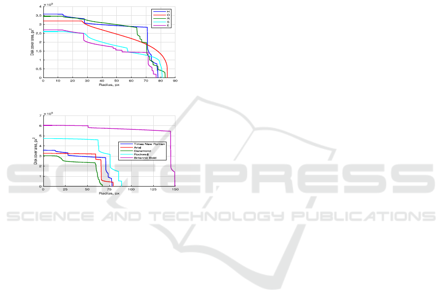
Example (Fig.12a) demonstrates width
diagrams for 5 letters of the Times New Roman
font, belonging to the word HORSE. The example
shows that the font characters have clearly
distinguishable individual portraits.
(a)
(b)
Figure 12: Width diagrams of different characters of the
same font (a) and the same character in different fonts (b).
Differences between the portraits of the same
letter H, typed by different fonts (Times New
Roman, Aria, Garamond, Britannic Bold,
Rockwell) are shown in next example (Fig.12b).
These diagrams are obtained for high-resolution
images, which are considered as reference samples.
To conduct the experiment under more realistic
conditions, reference images of 52 characters of the
Latin alphabet (26 uppercase and 26 lowercase
letters) for 1848 typefaces ParaType digital font
collection (Yakupov et al., 2015) have been
constructed. For the reference images the width
diagrams were obtained by the method described in
this article. To do this, each character was drawn
on a binary raster image on such a scale that the
height of a capital letter H was 1000 pixels. For
these images continuous skeletons were
constructed and their basis width histograms were
calculated with the radius step of 0.5 pixel.
For the same fonts the images of the characters
were obtained in a lower resolution, so that the
height of letter H was 100 and 70 pixels. For these
characters, width diagrams also were built. Step
radius in the calculation was 0.05 and 0.035 pixels,
respectively. These diagrams were normalized so
that they could be compared with the diagrams of
reference font characters. Normalization was done
by stretching the diagrams 10 times along the -
axis and 100 times along the -axis and 14.29
times along the -axis and 204.08 times along the
-axis for low resolutions of 100 and 70 pixels
respectively. As a result, all the normalized
diagrams used the same set of radius values.
Creating of the skeletons and the calculation of
width diagrams (for 52 glyphs of 1848 fonts) took
in total less than 4 minutes on the computer with
Intel® Core i5
TM
processor and 6GB of RAM
Further, for each font images of the 1000
common English words, random 30% of which were
converted to upper case, were composed from the
letters in low resolution. These images were used as
the test set. Next, the diagrams of the letters on test
images were compared with the diagrams of
reference images in
metric. As an integral font
similarity metric we use a linear combination of
distances between all characters present in the
word. The coefficients of the linear form for each
word were obtained by training on the entire set of
test fonts. In the experiment, we calculated the
distances for 52 letters between all pairs of 1848
typefaces, which took 18 minutes, and 1000 times
trained the linear form, which took 32 minutes.
This means that the time of the request – checking
the typeface in the basis of the references – is 2
seconds and most of this time is spent to training of
the linear form.
The experimental results showed that the font
recognition accuracy by one word at the resolution
of 100 was 91%, and at a resolution of 70 – more
than 81%. Using the imaginary word containing all
52 characters we achieved the accuracy of 97% and
95% respectively.
Thus, the experiment confirmed the efficiency
of the proposed method and showed its efficiency
on the practical task of comparing a large number
of images (1848184852) with a fairly high
recognition quality.
9 CONCLUSION
The proposed approach opens up new possibilities
for the use of highly efficient computational
geometry algorithms in image analysis and shape
recognition. The continuous model of width of
polygonal figures on the basis of the disk cover
allowed to make the decomposition of the original
Pattern Width Description through Disk Cover - Application to Digital Font Recognition
491

problem and reduce the computation to simple
geometric calculations.
The developed algorithm is the first to provide
accurate analytical representation of the width
distribution function of a polygonal figure. Raster
objects approximation with polygonal figures makes
it possible to use the method in the analysis and
recognition of images. The high efficiency of the
proposed method allows to compare and measure the
similarity of figures by their width in real-time
computer vision systems.
ACKNOWLEDGEMENTS
The work was funded by Russian Foundation of
Basic Research grant No. 14-01-00716.
REFERENCES
Maragos P., 1989. Pattern Spectrum and Multiscale Shape
Representation. In IEEE Trans. On Pattern Analysis
and Machine Intelligence, Vol. 11, №7, pp. 701–716.
Serra J., 1982. Image Analysis and Mathematical
Morphology, London: Academic Press.
Ramirez-Cortes, J.M., Gomez-Gil, P., Sanchez-Perez, G.,
Baez-Lopez, D., 2008. A Feature extraction method
based on the pattern spectrum for hand shape
biometry. In Proc. World Congress on Engineering
and Computer Science.
Vizilter Yu.V., Sidyakin S.V., 2012. Morphological
spectra [in Russian]. In Computer vision in control
systems 2012. Proceedings of the scientific-technical
conference, Moscow, 14–16 March, 2012. Pp. 234–
241.
Vizilter Yu.V., Sidyakin S.V., 2015. Comparison of
shapes of two-dimensional figures with the use of
morphological spectra and EMD metrics. In Pattern
Recognition and Image Analysis, Vol. 25, No. 3, pp.
365–372.
Lomov N.A, Mestetskiy L.M, 2016. Area of the disk cover
as an image shape descriptor. In Computer Optics, vol.
40(1), pp. 516-525.
Mestetskiy, L., Semenov, 2008. Binary image skeleton
continuous approach. VISAPP 2008 - 3rd
International Conference on Computer Vision Theory
and Applications, Proceedings 1, pp. 251-258.
Yakupov E., Petrova I., Fridman G., Korolkova A., Levin
B., 2015. PARATYPE Originals – Digital Typefaces.
Moscow, 2015.
VISAPP 2017 - International Conference on Computer Vision Theory and Applications
492
