
Riemannian Filters for Multi-variate Mesh Signals
Teodor Cioaca
1
, Bogdan Dumitrescu
1
and Mihai-Sorin Stupariu
2
1
University Politehnica of Bucharest, Bucharest, Romania
2
University of Bucharest, Bucharest, Romania
Keywords:
Graph Wavelets, Multi-variate Mesh Signals, Riemannian Mean Shift.
Abstract:
Designing filters over irregular non-Euclidean domains requires algorithms that take into account the intrinsic
curvature of these domains. We propose a new filtering method based on Riemannian weighted averages. The
resulting filters are non-Euclidean adaptations of the mean shift and blurring mean shift algorithms. We also
introduce a hybrid, efficient computing strategy by combining these iterative filtering methods with wavelet
multi-resolution editing. The applications of our filters include multi-variate mesh data smoothing, denoising,
attribute enhancement and curvature filtering.
1 INTRODUCTION
Filtering operations are essential tools of signal pro-
cessing. For signals sampled over 1-D and 2-D reg-
ular, flat domains the existing literature offers an ex-
tensive collection of filtering methods. In the case of
graphs and meshes, where the domain can be highly
irregular and intrinsically curved, it is not immedi-
ately possible to adapt and apply even the simpler
mean or Gaussian blurring filters. The main difficul-
ties stem from the fact that non-Euclidean domains
are no longer closed under linear combinations of
points.
In this work, we develop a solution for the numer-
ical evaluation of a mean shift filter on discretely sam-
pled 2-dimensional smooth Riemannian manifolds.
The principle we use to overcome the difficulties in
working on non-Euclidean spaces is to perform the
filter iterations in the local tangent space and then
project the result onto the underlying manifold. This
same strategy is used in the continuous case, in the
Weiszfeld algorithm (Aftab et al., 2015). We extend
the technique to meshes with per-vertex attributes.
This way, we design a family of mean shift algorithms
that function on curved domains, even under condi-
tions of heavy noise corruption.
1.1 Related Work
Since its introduction by (Fukunaga and Hostetler,
1975), there have been many attempts to adapt the
mean shift algorithm to geometrically complex do-
mains. (Yamauchi et al., 2005) use an Euclidean ver-
sion of the mean shift algorithm to segment meshes
by clustering faces. Although their method handles
geometry and normal orientations differently using
composite kernels, the filtered output is not guaran-
teed to lie on the same support mesh. (Zhang et al.,
2008) approach the segmentation problem via mean
shift by enhancing and filtering the per-vertex cur-
vature estimates. This solution does not evaluate
geodesic distances between samples, instead measur-
ing only topological distances. (Cerveri et al., 2012)
perform curvature mean shift filtering by also treat-
ing the feature spaces as entirely Euclidean where
the vertex coordinates and curvature values make up
the coordinates of a 4-dimensional space. (Shamir
et al., 2006) perform curvature mean shift using lo-
cal geodesic parameterizations. Still, their solution
requires rendering an entire mesh neighborhood to
a texture and performing image mean shift instead.
(Subbarao and Meer, 2009) correctly generalize the
mean shift filter to certain families of Riemannian
manifolds such as matrix Lie groups, Grassmann
manifolds, essential matrices and symmetric positive
definite matrices. (Cetingul and Vidal, 2009) propose
an intrinsic mean shift algorithm for Grassmann and
Stiefel manifolds. (Caseiro et al., 2012) introduce a
mapping of arbitrary Riemannian manifolds into a re-
producing kernel Hilbert space via a heat kernel ob-
taining a semi-intrinsic mean shift formulation.
(Solomon et al., 2014) introduce a generalized bi-
lateral and mean shift filtering framework for multi-
variate data on domains that admit a Laplacian oper-
228
Cioaca T., Dumitrescu B. and Stupariu M.
Riemannian Filters for Multi-variate Mesh Signals.
DOI: 10.5220/0006128602280235
In Proceedings of the 12th International Joint Conference on Computer Vision, Imaging and Computer Graphics Theory and Applications (VISIGRAPP 2017), pages 228-235
ISBN: 978-989-758-224-0
Copyright
c
2017 by SCITEPRESS – Science and Technology Publications, Lda. All rights reserved

ator. As such, their method can be applied to graphs,
meshes, images and point clouds. The main drawback
of this method is that the resulting mean shift algo-
rithm is not a sliding window mode-finding algorithm.
In essence, the framework computes a weighted aver-
age of the attributes with respect to the neighborhood
of a fixed sample on a curved domain. Opting for a
sliding window formulation leads to a better adaption
to the local structure of the data, as emphasized in
(Comaniciu and Meer, 2002).
1.2 Our Contributions
We generalize the works of (Pennec, 2006), (Fletcher
et al., 2008) and (Wang and Carreira-Perpin, 2010) to
generic mesh domains by eliminating the need of a
priori knowing a closed-form expressions for the ex-
ponential and logarithm maps on the underlying man-
ifold. In this work, we describe:
• a rigorous formulation for the mean shift imple-
mentation on general triangular meshes with both
geometry and attribute vertex data;
• a computation acceleration algorithm using a
graph-wavelet decomposition to filter a coarser
model and propagate changes through wavelet
synthesis, thus effectively reducing the size of the
problem.
The remainder of this paper is organized as fol-
lows. In section 2 we describe the mean shift filter and
how it can be extended to mesh domains. A hybrid
technique for accelerating the filter computations via
wavelet multiresolution is presented in section 3. We
further present mesh normal denoising and attribute
filtering applications in section 4 and conclude this
research in section 5.
2 FILTERING ON
NON-EUCLIDEAN DOMAINS
In this section we discuss the key ingredients required
to compute Riemannian weighted averages. Although
the main technique resembles the Euclidean case, the
computation on Riemannian manifolds is based on the
Weiszfeld algorithm (Aftab et al., 2015). For gen-
eral triangular meshes, the exponential and logarithm
maps are the only algorithm operations that cannot be
directly computed (since there is no closed-form ex-
pression available). Instead, we propose evaluating
the logarithm map using the geodesic polar coordi-
nates algorithm of (Melvær and Reimers, 2012). For
the exponential map, the straightest geodesics algo-
rithm described by (Polthier and Schmies, 1998) is
the most efficient choice. Both algorithms work on
triangular meshes and do not depend upon the genus
of the underlying mesh or upon the regularity of the
network.
2.1 Euclidean Mean Shift
Let x
i
∈ R
d
be a set of n data samples. It can be
assumed that the x
i
points are sampled from a ran-
dom variable whose density can be approximated us-
ing kernel estimators. The expression for this density
estimate at a point x ∈ R
d
is given by
ˆ
f
h,K
(x) =
c
K,d
nh
d
n
∑
i=1
k
x − x
i
h
2
!
, (1)
where h is the bandwidth parameter, k(·) is a kernel
profile function corresponding to a multi-variate ker-
nel K(x) := k (kxk
2
/h
2
) and c
K,d
is a normalization
constant.
The principle behind mean shift filtering is to re-
place each sample x with the closest mode of the prob-
ability density estimate. If
¯
x is such a mode, then
∇
ˆ
f
h,K
(
¯
x) = 0. The problem of finding
¯
x is usually
solved through an iterative gradient ascent process,
i.e.
x
(k+1)
← x
(k)
+ m
h,G
(x
(k)
), (2)
where
m
h,G
(x) =
n
∑
i=1
g
x−x
i
h
2
(x
i
− x)
n
∑
i=1
g
x−x
i
h
2
, (3)
with g(·) the kernel profile function of a multivariate
kernel G such that g(·) = −k
0
(·). In many practical
situations, the individual coordinates of the samples
have different interpretations. The most common ex-
ample is that of an image where spatial and range co-
ordinates are concatenated. Formally, x =
x
s
x
r
|
,
with x
s
∈ R
p
,x
r
∈ R
q
and p + q = d. Given the dif-
ferent semantics of these coordinates, a concatenated
kernel (as proposed by (Comaniciu and Meer, 2002))
can be used to achieve better bandwidth selection con-
trol. For spatial and range coordinates, equation (1)
becomes
ˆ
f
h
s,r
,K
(x) =
¯
C
n
∑
i=1
k
x
s
− x
i
s
h
s
2
!
k
x
r
− x
i
r
h
r
2
!
,
(4)
where
¯
C =
c
K,d
nh
p
s
h
q
r
and h
s
and h
r
are the spatial and
range bandwidth parameters.
2.2 Riemannian Mean Shift
We now consider the case when the sampled space
is inherently curve, i.e. {x
i
} ⊂ M for i ∈ 1,n and M
Riemannian Filters for Multi-variate Mesh Signals
229
a 2-dimensional Riemannian manifold embedded in
R
d
. Further, let us consider x
i
to be the vertices of a
mesh network. The iterative process in equation (2)
no longer moves the samples along the surface of the
domain manifold. Furthermore, the definition of the
kernel function must take into account the intrinsic
geodesic distance measured across the manifold. For
Riemannian manifolds, the gradient of the geodesic
distance function d(p,q) for p fixed is given by
∇
q
(d(p, q)) =
log
p
(q)
log
p
(q)
, (5)
where log
p
(q) is the logarithm map. As in the Eu-
clidean case, the samples may correspond to differ-
ent semantic spaces. In this situation, M is a sub-
manifold of M
s
× M
r
, where M
s
and M
r
are spatial
and range manifolds. An important result is that the
tangent space of the product can be decomposed as
a direct sum of the individual tangent planes, estab-
lishing a mapping T
x
s
(M
s
)⊕T
x
r
(M
r
) → T
x
(M
s
×M
r
).
If π
s
: M
s
×M
r
→ M
s
is the canonical projection, then
dπ
s
(x) is also a projection from T
x
(M
s
×M
r
) to T
x
s
M
s
.
Since the gradient of the density function is a vec-
tor in T
x
(M
s
×M
r
), then dπ
s
(x)
∇
ˆ
f
h
s,r
,K
(x)
∈ T
x
s
M
s
.
Further details on how to evaluate these quantities are
provided in the Appendix. Using this projection prin-
ciple, we now formulate the mean shift vector equiv-
alent of (3) in T
x
s
(M
s
), i.e.
m
h
s
,h
r
,G
s
(x) =
n
∑
i=1
g
d
2
s
(x
s
,x
i
s
)
h
2
s
k
d
2
r
(x
r
,x
i
r
)
h
2
r
log
x
s
(x
i
s
)
n
∑
i=1
g
d
2
s
(x
s
,x
i
s
)
h
2
s
k
d
2
r
(x
r
,x
i
r
)
h
2
r
.
(6)
Since the Riemannian mean shift vector lies in the
tangent space T
x
s
M
s
, we must project the result
back onto the manifold. This projection is achieved
through the exponential map, exp
x
s
(v
s
). We are now
able to assemble the mean shift algorithm for Rieman-
nian manifolds, which is similar to how the weighted
median is computed using the Weiszfeld algorithm
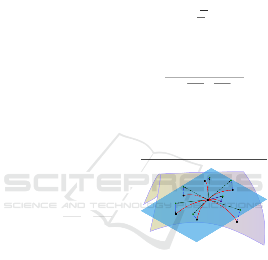
(see (Fletcher et al., 2009)). The iterative update
equation, illustrated in figure 1, is the following
x
(k+1)
← exp
x
(k)
m
h
s
,h
r
,G
s
(x
(k)
)
. (7)
In the above equation, the exponential maps canoni-
cally a vector from T
x
s
M
s
to a point on the M subman-
ifold of M
s
× M
r
.
The Riemannian mean shift presented in algo-
rithm 1 is formulated as a blurring filter. By setting
the total number of blurring passes N
p
= 1, we obtain
the classical mean shift algorithm. Performing more
than one filtering pass and using the filtered output as
the input of a next pass, the blurring effects become
Algorithm 1: Blurring Riemannian mean shift.
Require: {x
i
} ⊂ M, i ∈ 1,n .
Ensure: {y
i
} ⊂ M, ı ∈ 1,n, the modes of
ˆ
f
K,h
s
,h
r
cor-
responding to {x
i
}.
for pass ← 1 ...N
p
do
for i ← 1 . . . n do
y
(0)
i
← x
i
,k ← 0
repeat
m
h
s
,h
r
,G
s
(x) =
n
∑
j=1
g
d
2
s
(x
s
,x
j
s
)
h
2
s
k
d
2
r
(x
r
,x
j
r
)
h
2
r
log
x
s
(x
j
s
)
n
∑
j=1
g
d
2
s
(x
s
,x
j
s
)
h
2
s
k
d
2
r
(x
r
,x
j
r
)
h
2
r
y
(k+1)
i
← exp
y
(k)
i
m
h
s
,h
r
,G
∗
(y
(k)
i
)
k ← k +1
until ky
(k+1)
i
− y
(k)
i
k ≤ ε or k > k
max
y
i
← y
(k)
i
end for
for i ← 1 . . . n do
x
i
← y
i
end for
end for
T
p
M
x
x
i
log
x
x
i
exp
x
m
m
Figure 1: Computing the tangent-space mean shift vector
approximation via the log map, as described in equation (6).
The resulting mean shift vector is projected via the exp map
as detailed in equation (7).
more pronounced. The k
max
parameter is internally
used to control the maximum number of gradient as-
cent iterations, while ε is the error threshold used to
stop this refinement.
3 COMBINED WAVELET
FILTERING
Wavelet multiresolution analysis allows building a
hiearchical approximation of the initial mesh in a fine-
to-coarse fashion. Let M := M
L
M
L−1
... M
0
be the resulting chain of L successive approximations,
GRAPP 2017 - International Conference on Computer Graphics Theory and Applications
230

where M := M
L
is the initial mesh that is subjected
to the multiresolution analysis procedure. In general,
this process implies repeating the following decompo-
sition M
k+1
= M
k
∪
⊕
D
k
, where D
k
is the set of detail
vectors that are removed from M
k+1
in order to pro-
duce the lower resolution approximation, M
k
. Using
the lifting scheme, this analysis operation becomes
trivially invertible. The lifting scheme design de-
Algorithm 2: Hybrid wavelet-based filtering strategy.
Require: M = (V,E,F) high resolution mesh, L
number of intermediate approximations
Ensure:
¯
M :=
¯
M
L
¯
M
L−1
.. .
¯
M
0
a filtered hi-
erarchical approximation
for k ← n,1 do
M
k
= M
k−1
∪
⊕
D
k−1
end for
CALL algorithm 1 M
0
→
¯
M
0
for k ← 1,n do
¯
M
k
=
¯
M
k−1
∪
⊕
α
k−1
D
k−1
end for
veloped by (Cioaca et al., 2016) is a light-weight so-
lution for performing analysis on multi-variate mesh
data. Carrying out the intensive mean shift computa-
tions on the coarsest approximation, M
0
, we obtain a
new mesh,
¯
M
0
. We then recover the high resolution
model through wavelet synthesis. This is achieved
by adding back missing details with a certain cho-
sen amplitude, α
k
∈ R
+
. The synthesis thus con-
sists of update sequences
¯
M
k
=
¯
M
k−1
∪
⊕
α
k−1
D
k−1
,
where α
k−1
D
k−1
is the set of difference vectors uni-
formly scaled by the α
k−1
factor. This whole process
is sketched in algorithm 2.
4 RESULTS AND DISCUSSION
4.1 Mesh Smoothing Via Normal
Filtering
We test the non-linear filter through a series of
normal-based mesh smoothing experiments. We ap-
ply the mean shift algorithm, treating the per-vertex
normals as additional attribute data. Refining these
normals allows for smoothing and repairing the mesh.
The algorithm of (Lee and Wang, 2005) serves this
purpose by iteratively altering the vertex positions to
align the one-ring face normals with the filtered sam-
ples. While (Solomon et al., 2014) chose to treat face
normals separately, we have found that it is possible to
filter the per-vertex normals instead and approximate
the face normal by averaging the three normals of its
vertices. This choice eliminates the need of remesh-
ing the input model and allows treating normal infor-
mation as any kind of attribute data.
To ensure the exponential and logarithm map
computations are not influenced by the artificial geo-
metric noise, the base model was subjected to a Lapla-
cian smoothing pass using the method of (Taubin,
1995). We however note that the mean shift filter
was not found to lead to a significant degradation of
the normal field, but, when extending the geodesic
neighborhood radius, the exponential map samples
became unreliable. The Laplacian smoothed output
is solely used for computing the exponential and log-
arithm maps and does not constitute the input of the
algorithm described by (Lee and Wang, 2005).
The models used in our tests (also used in
(Solomon et al., 2014) and depicted in figure 2) were
rescaled to fit within the unit cube. The denoising ex-
periments were performed by artificially adding ver-
tex displacements having a uniform distribution of
magnitudes half the size of the average edge length.
This choice of the artificial noise distribution is iden-
tical to that proposed in (Solomon et al., 2014) and al-
lows for a qualitative assessment between the results
described in this work and our own experiments.
The methods selected for comparison are the com-
bined vertex and tangent plane projection feature
preserving smoothing of (Jones et al., 2003), the
prescribed mean curvature flow of (Hildebrandt and
Polthier, 2004), the bilateral normal filter of (Zheng
et al., 2011) and the bilateral and mean shift frame-
work of (Solomon et al., 2014).
To achieve normal-based mesh filtering we per-
formed three alternating passes of algorithm 1 and the
vertex relaxation routine of (Lee and Wang, 2005).
To penalize both normal dissimilarity and sample dis-
tance, we used the following kernel expression in
equation (6)
exp
−
d
2
(x
s
,x
i
s
)
2h
2
s
exp
−1
2h
2
r
(0.5 + 0.5n
x
|
n
x
i
)
2
,
(8)
where n
x
is the unit normal vector at a point x.
The mean shift is performed inside a geodesic ra-
dius r = 4AEL, using the bandwidth parameter values
h
s
= 3AEL, h
r
= 0.45, where AEL denotes the mesh
average edge length. The iteration count is controlled
by setting k
max
= 50 and ε = AEL/5.
The denoised models are depicted in figure 3.
Table 1 compares our method to several state-
of-the-art mesh denoising algorithms using the root
mean square distance, computed using MeshLab
(Cignoni et al., 2008)). Observing the smoothed
meshes (figure 3), we conclude that the filtering al-
gorithm of (Zheng et al., 2011) is more efficient
Riemannian Filters for Multi-variate Mesh Signals
231
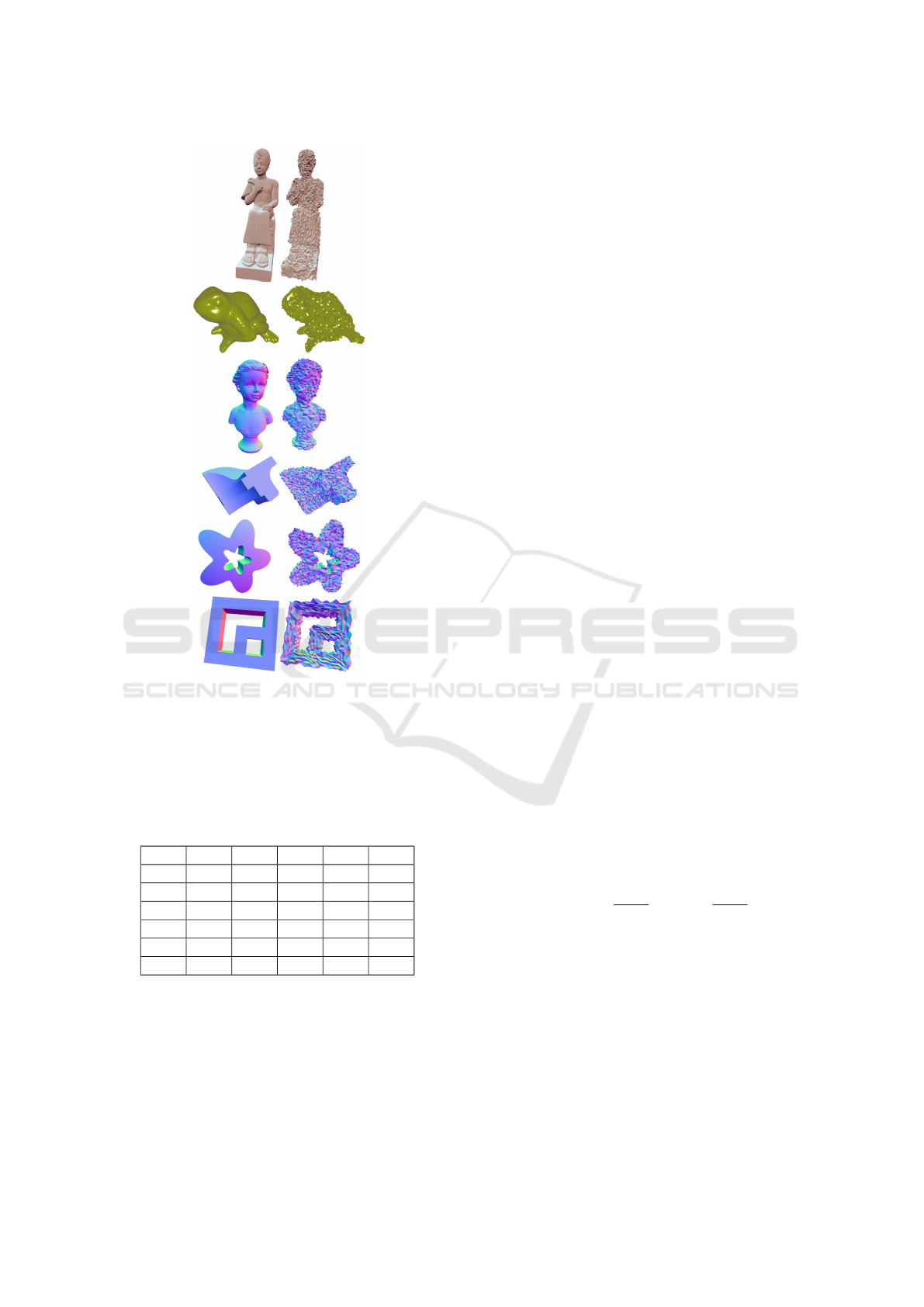
Figure 2: Mesh models with added uniform noise (vertex
displacements half the mean edge length).
Table 1: Root mean square distance values for the mesh de-
noising experiments (scaled by 10
2
). Models: (R)amesses,
(Fr)og, (B)ust, (F)andisk, (S)tar and (D)ouble torus. Meth-
ods, top to bottom: (Jones et al., 2003), (Hildebrandt and
Polthier, 2004), (Zheng et al., 2011), bilateral and mean
shift filters of(Solomon et al., 2014), our Riemannian mean
shift filter.
(R) (Fr) (B) (F) (S) (D)
0.36 0.36 0.47 0.58 0.44 1.2
0.34 - 0.52 0.47 0.34 0.45
0.23 0.30 0.39 0.33 0.55 0.47
0.24 0.27 0.40 0.38 0.41 0.5
0.24 0.31 0.35 0.31 0.41 0.42
0.26 0.24 0.41 0.35 0.35 0.44
than the methods of (Jones et al., 2003), (Hilde-
brandt and Polthier, 2004) and than the bilateral fil-
ter of (Solomon et al., 2014). The mean shift filter
of (Solomon et al., 2014) tends to produce smoother
meshes, with fewer isolated artifacts. Overall, our fil-
ter produces smooth output surfaces with a few per-
ceivable, low frequency noise artifacts. Compared to
other methods, the high frequency noise components
are suppressed. The visual quality and numerical re-
sults recommend our filtering technique for situations
where a unified filtering framework that can handle
both geometry and attribute smoothing tasks.
4.2 Combined Wavelet Attribute
Filtering
Given the iterative nature of the mean shift algorithm,
it is important to understand the computational com-
plexity of the underlying operations. The exponential
map can be found in linear time and is straightfor-
ward to compute. The logarithm map, on the other
hand, falls in the O(nlog(n)) family. Keeping a small
geodesic window radius helps reducing the impact on
scalability. If algorithm 2 is used, inputs with several
millions of samples can be efficiently handled.
4.2.1 Application to Terrain Modeling
In practice, large input models are commonplace.
For an applied proof of concept, we propose filter-
ing terrain models digitized from LiDAR scans. De-
noising or smoothing this type of data is a com-
mon GIS task, but the computations tend to be slow
given the size of the input. For our numerical ex-
periments we chose two terrain samples: one rep-
resenting a fragment of the Great Smoky Moun-
tains (having 270,000 points), obtained through the
http://www.opentopography.org/ portal, and an-
other one representing a fragment of the Romanian
Carpathian Mountains (having 11.8 million points),
obtained through a custom aerial scan. These models
include both geometric coordinates, as well as vegeta-
tion information in the form of a height offset (above
ground) between 0 and 30 meters and a class index
that ranges between the scalar values of 2 and 15.
To incorporate a spatial and range dissimilarity pe-
nalizing effect in the filter iteration, we opt for a prod-
uct of Gaussians kernel, i.e.
K
∗
(x) := exp
−
kx
s
k
2
2h
2
s
exp
−
kx
r
k
2
2h
2
r
. (9)
We ran the single-pass mean shift algorithm (MS) set-
ting the parameters h
s
= 8AEL, h
r
= 4, ε = AEL/20
and k
max
= 50. To achieve a blurring effect (BMS),
we set h
r
= 5AEL, h
s
= 5, ε = AEL/5 and k
max
= 5
and execute a sequence of 10 blurring passes inside
algorithm 1. We summarize the execution times of
both algorithm variations for the terrain models in ta-
ble 2 using different values for the number of levels
parameter, L, of algorithm 2.
Figure 4 illustrates the terrain models before and
after subjecting them to the combined wavelet and
GRAPP 2017 - International Conference on Computer Graphics Theory and Applications
232
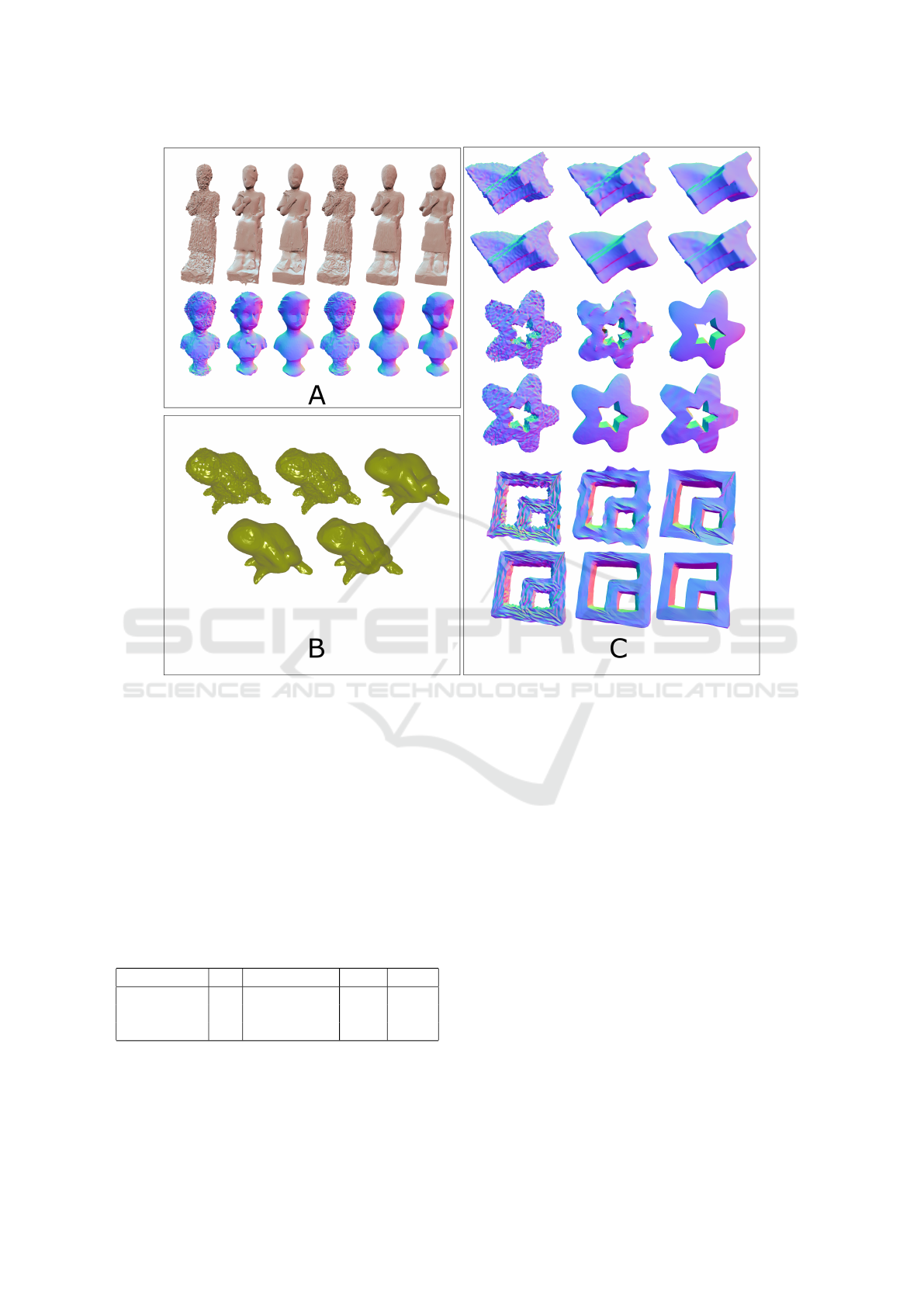
Figure 3: Denoising experiments. A: from left to right (Jones et al., 2003), (Hildebrandt and Polthier, 2004), (Zheng et al.,
2011), bilateral and mean shift of (Solomon et al., 2014) and our mean shift filter. B: from left to right and from top to bottom
(Jones et al., 2003), (Hildebrandt and Polthier, 2004), (Zheng et al., 2011), mean shift of (Solomon et al., 2014) and our mean
shift filter. C: from left to right and from top to bottom (Jones et al., 2003), (Hildebrandt and Polthier, 2004), (Zheng et al.,
2011), bilateral and mean shift of (Solomon et al., 2014) and our mean shift filter.
Riemannian mean shift filters (i.e. algorithms 1 and
2). Setting the α
k
= 1 is equivalent to adding back the
missing geometry and attribute details, while setting
α
k
= 0 suppresses the higher frequency components,
including noise. In our experiments, we filter and de-
noise these models by completely suppressing the de-
tails. The recovered, high resolution models exhibit
smoother vegetation boundary contours.
Table 2: Algorithm benchmarks for the LiDAR point sets.
Model L Vertex count MS BMS
Frog 2 5242 5s 16s
Smoky 6 40438 40s 120s
Carpathians 12 229095 260s 780s
The execution times of our algorithms, detailed
in table 2, are sensibly lower than those reported by
(Shamir et al., 2006). In total, the authors report
an execution time of 10 minutes for a mesh with
20,000 vertices on a 2GHz machine. In our set-up,
we have benchmarked single-threaded implementa-
tions of both algorithms. The machine used to evalu-
ate the performance on the datasets from table 2 was
running at a frequency of 3GHz. All algorithms were
implemented in standard C++.
4.2.2 Curvature Filtering
Curvature filtering and curvature-based segmentation
are other common mesh processing applications. In
our last experiment, we compute the absolute discrete
curvature and map it to a vertex color attribute us-
ing MeshLab (Cignoni et al., 2008). We then run the
filtering algorithm on the bust and frog meshes, set-
ting the α
k
factors from algorithm 2 to 0, thus com-
pletely suppressing the higher frequency information.
Both models are subjected to a sequence of only 2
wavelet analysis steps, reducing the vertex count to
approximately 56% of the initial model. More specif-
Riemannian Filters for Multi-variate Mesh Signals
233
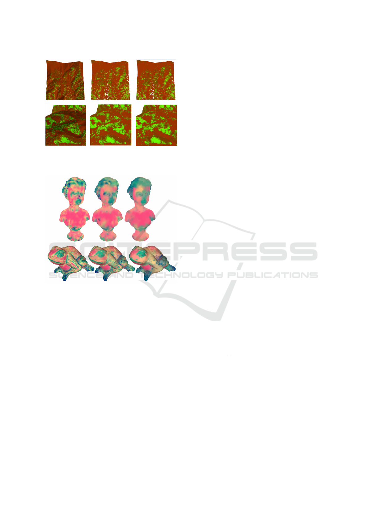
Figure 4: Rows: the Smoky Mountains fragment and the
Carpathian Mountains fragment. Columns, left to right:
original data, low resolution filtered with mean shift, low
resolution filtered with blurring mean shift.
Figure 5: Curvature filtering using algorithm 2 with α
k
=
0. Left to right: initial, mean shift and blurring mean shift
filtered color-coded absolute curvature values.
ically, the frog model is reduced from 9815 points
to 5242 points. The algorithm parameters are h
s
=
3AEL, h
r
= 0.25 for the single pass mean shift and
h
s
= 5AEL , h
r
= 0.1 for the blurring mean shift with
10 passes. The curvature filtering results for the frog
and bust models are shown in figure 5.
5 CONCLUSIONS
The filter described in our work is a rigorous discrete
formulation of the mean shift method on Riemannian
manifolds. We are not aware of any to-date adap-
tations that are set up in general context of meshes
viewed as sampled Riemannian manifolds. Our ap-
proach does not require prior knowledge about the
characteristics of the manifold subjected to these fil-
ters (e.g. the exponential and logarithm maps need not
have a known closed-form expression). Furthermore,
the iterative process considers both the geometry and
connectivity of the underlying mesh, guaranteeing the
filters output samples that lie on the surface, along
geodesic paths that originate from a seed point. This
is an improvement over existing literature where there
is either no such a guarantee or where the iterations
are performed in a Euclidean fashion.
Reducing the size of the input through wavelet
analysis is an effective compromise that allows per-
forming the time-consuming filtering operations on a
coarse approximation. In our experiments, we have
successfully recovered sets subjected to up to 12 con-
secutive analysis passes, combining the effects from
both the low resolution mean filter and from suppress-
ing the high frequency details (which often are af-
fected by noise).
The main limitations are the need to use pre-
smoothed geometry for robust exponential map eval-
uations and the subtle data dependency imposed by
the selection of the bandwidth parameters h
s
and h
r
.
Since our mean shift implementation also requires
projecting the gradient of the density function onto
the tangent space of the spatial coordinate manifold,
the question whether performing the filter iterations
on the entire tangent space product can improve the
results represents a research direction. We thus con-
sider these points to constitute directions of improve-
ment and future research.
ACKNOWLEDGEMENTS
The authors would like to thank Dr. Justin Solomon
for providing numerical results for the mesh smooth-
ing methods presented in (Jones et al., 2003), (Hilde-
brandt and Polthier, 2004), (Zheng et al., 2011) and
(Solomon et al., 2014).
This work was supported by the Swiss Enlarge-
ment Contribution in the framework of the Romanian-
Swiss Research Program, project WindLand, project
code: IZERZO 142168/1 and 22 RO-CH/RSRP.
REFERENCES
Aftab, K., Hartley, R., and Trumpf, J. (2015). General-
ized Weiszfeld algorithms for Lq optimization. IEEE
Transactions on Pattern Analysis and Machine Intel-
ligence, 37:728–745.
Caseiro, R., Henriques, J. a. F., Martins, P., and Batista, J.
(2012). Semi-intrinsic mean shift on riemannian man-
ifolds. In Proceedings of the 12th European Confer-
ence on Computer Vision - Volume Part I , ECCV’12,
pages 342–355, Berlin, Heidelberg. Springer-Verlag.
GRAPP 2017 - International Conference on Computer Graphics Theory and Applications
234

Cerveri, P., Manzotti, A., Marchente, M., Confalonieri, N.,
and Baroni, G. (2012). Mean-shifted surface curva-
ture algorithm for automatic bone shape segmentation
in orthopedic surgery planning: a sensitivity analy-
sis. Computer Aided Surgery, 17(3):128–141. PMID:
22462564.
Cetingul, H. E. and Vidal, R. (2009). Intrinsic mean shift
for clustering on stiefel and grassmann manifolds. In
2009 IEEE Conference on Computer Vision and Pat-
tern Recognition, pages 1896–1902.
Cignoni, P., Corsini, M., and Ranzuglia, G. (2008). Mesh-
Lab: an Open-Source 3D Mesh Processing System.
Ercim News, 2008.
Cioaca, T., Dumitrescu, B., and Stupariu, M.-S. (2016).
Graph-based wavelet representation of multi-variate
terrain data. Computer Graphics Forum, 35(1):44–58.
Comaniciu, D. and Meer, P. (2002). Mean shift: A robust
approach toward feature space analysis. IEEE Trans.
Pattern Anal. Mach. Intell., 24(5):603–619.
Fletcher, P. T., Venkatasubramanian, S., and Joshi, S.
(2008). Robust statistics on riemannian manifolds via
the geometric median. In Computer Vision and Pat-
tern Recognition, 2008. CVPR 2008. IEEE Confer-
ence on, pages 1–8.
Fletcher, P. T., Venkatasubramanian, S., and Joshi, S.
(2009). The geometric median on riemannian mani-
folds with application to robust atlas estimation. Neu-
roImage, 45(1, Supplement 1):S143 – S152. Mathe-
matics in Brain Imaging.
Fukunaga, K. and Hostetler, L. (1975). The estimation of
the gradient of a density function, with applications in
pattern recognition. IEEE Transactions on Informa-
tion Theory, 21(1):32–40.
Hildebrandt, K. and Polthier, K. (2004). Anisotropic Fil-
tering of Non-Linear Surface Features. Computer
Graphics Forum, 23:391–400.
Jones, T. R., Durand, F., and Desbrun, M. (2003). Non-
iterative, feature-preserving mesh smoothing. ACM
Trans. Graph., 22(3):943–949.
Lee, K. and Wang, W. (2005). Feature-preserving mesh
denoising via bilateral normal filtering. In 9th In-
ternational Conference on Computer-Aided Design
and Computer Graphics, CAD/Graphics 2005, Hong
Kong, China, 7-10 December, 2005, page 6.
Melvær, E. L. and Reimers, M. (2012). Geodesic polar co-
ordinates on polygonal meshes. Computer Graphics
Forum, 31(8):2423–2435.
Pennec, X. (2006). Intrinsic statistics on riemannian man-
ifolds: Basic tools for geometric measurements. J.
Math. Imaging Vis., 25(1):127–154.
Polthier, K. and Schmies, M. (1998). Straightest Geodesics
on Polyhedral Surfaces, pages 135–150. Springer
Berlin Heidelberg.
Shamir, A., Shapira, L., and Cohen-Or, D. (2006). Mesh
analysis using geodesic mean-shift. Vis. Comput.,
22(2):99–108.
Solomon, J., Crane, K., Butscher, A., and Wojtan, C.
(2014). A general framework for bilateral and mean
shift filtering. ArXiv e-print 1405.4734, 32.
Subbarao, R. and Meer, P. (2009). Nonlinear mean shift
over riemannian manifolds. International Journal of
Computer Vision, 84(1):1–20.
Taubin, G. (1995). Curve and surface smoothing without
shrinkage. In Proceedings of the Fifth International
Conference on Computer Vision, ICCV ’95, pages
852–852, Washington, DC, USA. IEEE Computer So-
ciety.
Wang, W. and Carreira-Perpin, M. . (2010). Manifold blur-
ring mean shift algorithms for manifold denoising.
In Computer Vision and Pattern Recognition (CVPR),
2010 IEEE Conference on, pages 1759–1766.
Yamauchi, H., Lee, S., Lee, Y., Ohtake, Y., Belyaev, A., and
Seidel, H.-P. (2005). Feature sensitive mesh segmen-
tation with mean shift. In Proceedings of the Inter-
national Conference on Shape Modeling and Applica-
tions 2005, SMI ’05, pages 238—245, Washington,
DC, USA. IEEE Computer Society.
Zhang, X., Li, G., Xiong, Y., and He, F. (2008). 3D Mesh
Segmentation Using Mean-Shifted Curvature, pages
465–474. Springer Berlin Heidelberg, Berlin, Heidel-
berg.
Zheng, Y., Fu, H., Au, O. K.-C., and Tai, C.-L. (2011).
Bilateral normal filtering for mesh denoising. IEEE
Transactions on Visualization and Computer Graph-
ics, 17(10):1521–1530.
APPENDIX
We evaluate the gradient of (4) on M
s
× M
r
∇
ˆ
f
h
s,r
,K
(x) =
n
∑
i=1
k
0
d
2
s
(x
s
,x
i
s
)
h
2
s
k
d
2
r
(x
r
,x
i
r
)
h
2
r
2
h
2
s
log
x
i
s
(x
s
),0
r
+
n
∑
i=1
k
d
2
s
(x
s
,x
i
s
)
h
2
s
k
0
d
2
r
(x
r
,x
i
r
)
h
2
r
2
h
2
r
0
s
,log
x
i
r
(x
r
)
.
(10)
Through projection onto T
x
s
M
s
we obtain
dπ
s
(x)
∇
ˆ
f
h
s,r
,K
(x)
=
n
∑
i=1
k
0
d
2
s
(x
s
,x
i
s
)
h
2
s
k
d
2
r
(x
r
,x
i
r
)
h
2
r
2
h
2
s
log
x
i
s
(x
s
). (11)
Riemannian Filters for Multi-variate Mesh Signals
235
