
A Multiclass Anisotropic Mumford-Shah Functional for Segmentation of
D-dimensional Vectorial Images
J. F. Garamendi
1
and E. Schiavi
2
1
Departament de Tecnologies de la Informaci
´
o i les Comunicacions, Universitat Pompeu Fabra, Barcelona, Spain
2
Departamento de Matem
´
atica Aplicada, Ciencia e Ingenieria de los Materiales y Tecnolog
´
ıa Electr
´
onica,
Universidad Rey Juan Carlos, M
´
ostoles, Spain
jf.garamendi@upf.edu, emanuele.schiavi@urjc.es
Keywords:
Multi-channel Image Segmentation, Variational Methods, Mumford-Shah.
Abstract:
We present a general model for multi-class segmentation of multi-channel digital images. It is based on the
minimization of an anisotropic version of the Mumford-Shah energy functional in the class of piecewise con-
stant functions. In the framework of geometric measure theory we use the concept of common interphases
between regions (classes) and the value of the jump discontinuities of the (weak) solution between adjacent
regions in order to define a minimal partition energy functional. The resulting problem is non-smooth and
non-convex. Non-smoothness is dealt with highlighting the relationship of the proposed model with the well
known Rudin, Osher and Fatemi model for image denoising when piecewise constant solutions (i.e partitions)
are considered. Non-convexity is tackled with an optimal threshold of the ROF solution which we which gen-
eralize to multi-channel images through a probabilistic clustering. The optimal solution is then computed with
a fixed point iteration. The resulting algorithm is described and results are presented showing the successful
application of the method to Light Field (LF) images.
1 INTRODUCTION
Image segmentation is, possibly, one of the most im-
portant steps of any image analysis, recognition or
image quantification process. Among the most es-
tablished methods, minimization of a feasible energy
functional has proven to be an efficient, accurate and
sound based mathematical framework for digital im-
age processing. A key stone in image segmentation
is the celebrated Mumford and Shah model (Mum-
ford and Shah, 1989) which is a piecewise model pro-
ducing a partition (segmentation) of a digital image.
Several mathematical and computational difficulties
arise when this model is considered. Convex formu-
lations have been proposed for solving a more general
model in terms of multi-labelling problems, (Pock
et al., 2009) and (Brown et al., 2011). A simplified
version of the Mumford and Shah model in a curve
evolution framework (level sets) is also considered in
(Chan and Vese, 2001). Their proposal amounts to
consider a coupled system of parabolic equations and,
as such, it presents a strong dependency on the initial-
ization of the numerical scheme and a extremely low
stabilization rate to the steady state solution. Also,
this model do not properly takes account of the lo-
cal inter-phases between adjacent classes (some are
counted twice and some are missed).
The framework we propose is a generalization of
the model for binary (2-classes) segmentation of 2D
grayscale images proposed by Osher and Vese (Os-
her and Paragios, 2003). We use the concept of
weights for the inter-phase lengths introduced for bi-
nary segmentation and we generalize it to M-Classes
segmentation on D-Dimensional vectorial images.
This generalization leads to an anisotropic version
of the Mumford-Shah model (hereafter AMS model).
Moreover, we show that the resulting AMS model for
multi-class multi-channel segmentation has the same
minimum as the vectorial version of the celebrated
Rudin, Osher and Fatemi (Rudin et al., 1992) de-
noising model (from now on VROF model) when re-
stricted to (minimized in) the set of piecewise con-
stant functions (which are SBV (Ω) functions). In
fact the energy of the two functionals is exactly the
same when this set is considered for minimization.
In turn this allows to solve the segmentation problem
using the well-established theory for the ROF model
where existence and uniqueness was proved (Cham-
bolle and Lions, 1997) and for which efficient nu-
merical schemes where developed (Chambolle, 2004;
468
Garamendi J. and Schiavi E.
A Multiclass Anisotropic Mumford-Shah Functional for Segmentation of D-dimensional Vectorial Images.
DOI: 10.5220/0006127804680475
In Proceedings of the 12th International Joint Conference on Computer Vision, Imaging and Computer Graphics Theory and Applications (VISIGRAPP 2017), pages 468-475
ISBN: 978-989-758-225-7
Copyright
c
2017 by SCITEPRESS – Science and Technology Publications, Lda. All rights reserved

Garamendi et al., 2013; Chambolle and Pock, 2011).
Possible applications of the proposed multiclass
model are segmentation of a given Optical Flow,
which is a 2D vectorial field, multimodal magnetic
resonance image, considering each modality as a sin-
gle channel, and in general multiclass segmentation
task. In this work, as a specific application of the
above general setting, we consider Light Field images
(LF) partition. There is a growing interest for light
field imaging applied to computer vision due to the
new hand-held cameras such as Lytro
1
or Raytrix
2
.
In fact, compared to conventional imaging, light field
imaging increases the directional information of the
scene. Plenoptic cameras (Lippman, 1908; Ng, 2006;
Ng et al., 2005; Perwass and Wietzke, 2010) capture
LF images from scene keeping the light direction in-
formation. The purpose of this cameras is capturing
the amount of light (radiance) traveling along each ray
that intersects the sensor. So, for each spatial position
in the 2-D space of the sensor, it stores the amount of
light coming from a certain space directions. So one
acquisition, or data set, has the information about how
the scene appears from a certain number of possible
viewpoints. More details can be found in (Wanner
et al., 2013a), (Reddy et al., 2013).
The mathematical modeling of the light filed im-
ages is usually done considering two planes of R
2
.
One of them defines the spatial coordinates in a sin-
gle view and the other one defines the view itself. Let
Ω ⊂ R
2
and Π ⊂ R
2
be bounded Lipschitz domains
representing the spatial image domain and the angu-
lar domain respectively, and let f be a multi-channel
data. The LF image can be modeled as the 4-D func-
tion
f : Ω × Π → R
M
,
( ¯p, ¯q) 7→ f( ¯p, ¯q)
where ¯p := (x,y) ∈ Ω and ¯q := (s,t) ∈ Π represent co-
ordinate pairs in the sensor plane spatial domain and
in the view angular domain respectively. This pro-
vides a model of a lightfield color image as a vecto-
rial 4D function, in such a way f(x, y,s,t) represents
the color (M = 3 in the case of RGB color images) at
pixel (x,y) corresponding to ray (s,t).
The structure of LF images allows for a very pre-
cisely disparity map computation with a very small
cost (Wanner et al., 2013b), so one can assumes that
this information is available as an additional feature to
the intensity (gray) color, making this modality of im-
age very well suited to segmentation. In this case, for
a color image in a RGB color space, M = 4, the three
1
www.lytro.com
2
www.raytrix.de
first components corresponding to color information
and the fourth to depth information. Notice that the
user can add other information to the channels as for
example local variance, texture, etc. This vectorial
4D dimensional structure of the images (color com-
ponents and depth) allows to test the model presented
in this work.
2 NOTATION AND DEFINITIONS
Let Ω ⊂ R
D
be a bounded Lipschitz domain repre-
senting the digital image domain and let f : Ω ⊂ R
D
→
R
M
be a given D-dimensional noisy image represent-
ing the data, where M = 1 for scalar images and M > 1
for vector valued (multichannel) images. As usual in
image processing we assume f ∈ [L
∞
(Ω)]
M
, i.e. f es-
sentially bounded.
Given an image and chosen the number N ≥ 2
of classes into which we wish to partition the given
image, the segmentation problem can be formulated
as the determination of a partition of the domain Ω
into a collection of sets
{
Ω
i
}
i=1..N
of finite perime-
ter (Cacciopoli sets) in Ω such that no overlap and
no vacuum can occur, e.g. Ω
i
∩ Ω
j
=
/
0, i 6= j, Ω =
S
N
i=1
Ω
i
∪ Γ
i
where the boundary of each class is de-
noted by Γ
i
= ∂Ω
i
∩Ω. Given a partition P(Ω) we de-
fine
¯
χ = (χ
i
), i = 1..N as the associated vectorial char-
acteristic function. For almost every point x ∈ Ω
i
⊂ Ω
we have
¯
χ : Ω → R
N
,
¯
χ(x) = ¯e
i
where ¯e
i
is a vec-
tor of the canonical base of R
N
. Notice that the di-
mension of
¯
χ depends on the number of classes and
it is independent from number of channels M. Also
N
∑
i=1
χ
i
(x) = 1,a.e.x ∈ Ω.
For a given vector valued function u : Ω → R
M
the vectorial TV norm, denoted as TV, is defined by
the finite positive measure (Ambrosio et al., 2000;
Bresson and Chan, 2008)
|Du|(Ω) =
Z
Ω
|Du|
.
= sup
P∈K
Z
Ω
hu,∇ · Pidx
(1)
where P : Ω → R
M×D
is a matrix dual function,
∇· is the divergence operator and the product h.,.i
is the Euclidean scalar product defined as hv,wi
.
=
∑
M
i=1
hv
i
,w
i
i from where hu,∇ · Pi =
∑
M
i=1
hu
i
,∇ · p
i
i.
The set K of functions of the dual variable P is
K
.
=
P ∈ C
1
c
Ω;R
M×D
: |P| ≤ 1
(2)
where | · | is the L
2
norm such that |P| =
q
∑
M
i=1
hp
i
,p
i
i.
A Multiclass Anisotropic Mumford-Shah Functional for Segmentation of D-dimensional Vectorial Images
469

Setting M = 1 and denoting the dual variable P in
vectorial form p (scalar case) we can use (1) to define
the perimeter of each subset Ω
i
of the partition in form
(Klann and Ramlau, 2013):
per(Ω
i
)
.
= |Dχ
i
|(Ω) =
Z
Ω
|Dχ
i
| = TV(χ
i
) = (3)
sup
p∈K
Z
Ω
χ
i
∇ · pdx
= sup
p∈K
Z
Ω
i
∇ · pdx
= |Γ
i
| (4)
where χ
i
is the characteristic function of the set Ω
i
and TV denotes the (scalar) Total Variation operator.
As a key feature of our framework we introduce
the concept and notation for the common interface be-
tween subsets Ω
i
of the partition P(Ω) of Ω. This pro-
vides a finer decomposition of the TV functional de-
fined in (1) into common inter-phases which recover
the discontinuity set of the solution weighting our be-
lieving of the classification through the strength of the
boundary (the jump of the solution). Sharp transi-
tions are then proportionally weighted and properly
(locally) considered. For this some notations are in-
troduced below.
Let Γ =
S
N
i=1
Γ
i
be the (discontinuity) jump set of
the solution u defined through a partition and let Γ
i
=
S
N
j=1
Γ
i j
, i 6= j, be the inter-phase (perimeter) of class
i, i.e the boundary of the class Ω
i
. Let moreover Γ
i j
to
denote the local inter-phases between the classes Ω
i
and Ω
j
where the length of the inter-phases is defined
as
|
Γ
|
=
Z
Γ
dH
D−1
(5)
|
Γ
i
|
=
Z
Γ
i
dH
D−1
(6)
Γ
i j
=
Z
Γ
i j
dH
D−1
(7)
The perimeter
|
Γ
i
|
can be computed summing up
the contribution of all the common interfaces between
the different classes of the partition
per(Ω
i
) = |Γ
i
| =
∑
i6= j
|Γ
i j
| (8)
that is the D − 1-dimensional Hausdorff measure
(|
/
0| = 0) of the (reduced) boundary of Ω
i
. Obviously
|Γ
i j
| = |Γ
ji
|.
Given a partition P(Ω) we define
¯
χ = (χ
i
), i =
1..N as the associated vectorial characteristic func-
tion. In this setting a vectorial piecewise constant
function u : Ω ⊂ R
D
→ R
M
taking exactly N differ-
ent positive values determined by a N-classes parti-
tion P(Ω) and coefficient matrix C ∈ R
M×N
, is deter-
mined via the vectorial mapping
F : P(Ω) × R
M×N
→ [L
∞
(Ω)]
M
(9)
in form u = F(
¯
χ,C)
.
= C
¯
χ. We can evaluate at each
pixel x ∈ Ω using this mapping in form F(x) : R
N
×
R
M×N
→ R
M
to have
u(x) = F(x) = F(
¯
χ(x),C)
.
= C
¯
χ(x) = C ¯e
i
= ¯c
i
∈ R
M
(10)
where i ∈ {1..N} is such that x ∈ Ω
i
. In other words
this vectorial mapping selects the vector column ¯c
i
of
the matrix C corresponding to the class Ω
i
to which
the pixel x ∈ Ω belongs. To each pixel corresponds
exactly only one column which is a vector of con-
stants which measure the sharpness of the boundary
depending on the jump of the solution at the local in-
terfaces. In fact there is a different jump at any local
inter-phase. Notice that the dimension of the partition
only depends on the number of classes N into which
we classify (segment) the image domain Ω and do not
depends on the number of channels M.
As example, for the simplest case of binary seg-
mentation (N = 2) of gray level scalar images (M = 1)
the associated coefficient matrix is simply C = ¯c =
(c
1
,c
2
) ∈ R
1×2
and we look for a piecewise constant
(binary) function in form
u = F(
¯
χ, ¯c)
.
= ¯c ·
¯
χ = c
1
χ
1
+ c
2
χ
2
(11)
where χ
1
and χ
2
= 1 − χ
1
are the characteristic func-
tions of the binary partition P(Ω) = {Ω
1
,Ω
2
}.
3 SEGMENTATION MODEL
In this section we propose the generalization of the
anisotropic version of the Mumford Shah functional,
for multi-class segmentation of multichannel images.
Its minimization leads to find a region-based segmen-
tation defined in the image domain Ω by a piecewise
constant function u = F(
¯
χ,C) = C
¯
χ into exactly N-
classes obtained from multichannel data f. For that
we propose to minimize the following energy func-
tional:
J(C,Γ) =
N−1
∑
i=1
N
∑
j=i+1
|c
j
−c
i
|
Γ
i j
+
1
2λ
Z
Ω
(C
¯
χ − f)
2
dx
(12)
where vectors c
i
∈ R
M
, i = 1..N are positive columns
vectors of the coefficient matrix C ∈ R
M×N
, f ∈
[L
∞
(Ω)]
M
is the given (noisy) vector valued image
and λ ∈ R
+
is a weighting parameter that acts as a
trade-off between the fidelity to the data and the reg-
ularity of the solution, i.e. the smaller the lambda is,
the less regular the solution will be.
VISAPP 2017 - International Conference on Computer Vision Theory and Applications
470

Finally, for piecewise constant functions u = C
¯
χ
the last term verifies
||
u − f
||
2
[L
2
(Ω)]
M
=
Z
Ω
|u − f|
2
dx =
Z
Ω
(C
¯
χ − f)
2
dx
(13)
and models the L
2
fidelity norm measuring the likeli-
hood of the data f assuming a Gaussian mixture dis-
tribution of the colors.
As example, for the simplest case of binary seg-
mentation (N = 2) of gray level scalar images (M =
1), we recover the model proposed in Osher and Vese
in (Osher and Paragios, 2003), that is a modified ver-
sion of the Chan-Vese functional (Chan and Vese,
2001) in which the length term is weighted by the
jump |c
2
− c
1
|, resulting in the following functional
J(C,Γ) = |c
2
− c
1
|
Z
Γ
dH
1
+
1
2λ
Z
Ω
1
|c
1
− f |
2
dx
+
1
2λ
Z
Ω
2
|c
2
− f |
2
dx (14)
where Γ is the unique common interface of the parti-
tion Γ = Γ
12
= Γ
21
.
A fundamental point is that this energy functional
can be written as the Rudin-Osher-Fatemi denoising
model (Rudin et al., 1992)
J(u) =
Z
Ω
|Du| +
1
2λ
Z
Ω
|u − f |
2
dx (15)
when its minimization is constrained to binary piece-
wise constant functions (Osher and Paragios, 2003)
and where we denoted as Du the generalized gradient
of u and with
Z
Ω
|Du| the total variation of u. Note
in J(C,Γ) that the minimization relates the disconti-
nuity set of the solution Γ with its length through the
TV operator. The term |c
2
− c
1
| is a weighting factor
defined by the partition in which the optimal constants
can be explicitly computed. This is not true anymore
when multichannel (M > 1) data are considered and a
coupling is present. A non-linear system of equations
has to be solved.
The key observation, first obtained in Chambolle
(Chambolle and Darbon, 2008), when studying the
Chan, Essedoglu, Nikolova model (Nikolova et al.,
2006) and here generalized to the multi-class multi-
channel framework, is that the functionals 12 and 15
are the same when restricted to piecewise constant so-
lutions. In fact we have the following theorem:
Theorem. Let N and λ be positive fixed parameters
and let Ω ⊂ R
D
be a given bounded open domain rep-
resenting the image domain. Let f ∈ L
∞
(Ω)
M
be a
vectorial data function M ≥ 1 where each scalar com-
ponent f
i
(x) : Ω → R represents a channel. Let u be
a vector valued piecewise constant function such as
u =
¯
F(
¯
χ,C) = C
¯
χ obtained from multichannel data f.
Then, the functional (12) coincides with the vec-
torial version of the ROF energy functional
J(u) =
Z
Ω
|Du| +
1
2λ
||
u − f
||
2
L
2
(Ω;R
M
)
(16)
Proof. Using the geometric measure theory of Am-
brosio, Fusco y Pallara (Ambrosio et al., 2000) as
well as the vectorial approach of Bresson, (Bresson
and Chan, 2008) the Total variation term TV(u) =
Z
Ω
|Du| in the functional (16) can be decomposed in
form:
Z
Ω
|Du| =
Z
Ω
|∇u|dx + |D
c
u|(Ω) +
Z
Γ
|u
+
− u
−
|dH
D−1
,
where ∇u denotes the Lebesgue part of the gradient
of u, the term D
c
u is the Cantor part of the measure
Du and Γ, as before, is the set of jumping points of u
being u
+
, u
−
the jump functions. The two first terms
vanish since u is piecewise constant and u ∈ SBV(Ω)
(the space of Special Bounded Variation functions de-
fined in (Ambrosio et al., 2000)). As a consequence
it has no Cantor part and the only contribution to the
energy is provided by the jump of the solution at the
local inter-phases Γ
i j
. We then have:
R
Ω
|Du| =
R
Γ
|u
+
− u
−
|dH
D−1
=
∑
N−1
i=1
∑
N
j=i+1
R
Γ
i j
|c
j
− c
i
|dH
D−1
=
∑
N−1
i=1
∑
N
j=i+1
|c
j
− c
i
|
R
Γ
i j
dH
D−1
=
∑
N−1
i=1
∑
N
j=i+1
|c
j
− c
i
||Γ
i j
|
(17)
As a straightforward consequence of the above
theorem, fixing the number N of classes into which
we wish to divide the image domain, the minimiza-
tion of the energy functional (16) restricted to the set
S of vectorial piecewise constant functions
S =
(
u = C
¯
χ/ c
i
∈ R
M
,
N
∑
i=1
χ
i
(x) = 1, a.e.x ∈ Ω
)
with S ⊂ BV(Ω; R
M
), is equivalent to the minimiza-
tion of the proposed energy functional (12). In both
cases the optimization problem is non-convex be-
cause the set of partitions of exactly N-classes, in
A Multiclass Anisotropic Mumford-Shah Functional for Segmentation of D-dimensional Vectorial Images
471

which we look subsets of R
N
, is a non-convex col-
lection (Nikolova et al., 2006). Nevertheless is well
known that the ROF model has exactly one solution
(a global minimum of the energy functional) when
minimized in the larger space of Bounded Variation
BV(Ω). So, in order to solve a convex problem,
we propose to minimize (16), over the larger space
BV(Ω;R
M
). The solution is now allowed to take val-
ues on the continuous interval [0,1]
M
and we obtain a
solution in set S using a thresholding step based on a
maximum probability criterion. The numerical solu-
tion of the ROF model can be obtained using known
algorithms such as dual, staggered or primal-dual al-
gorithms (Chambolle, 2004; Garamendi et al., 2013;
Chambolle and Pock, 2011). Finally the optimal con-
stants of the selected piecewise solution are computed
with a simple fixed point algorithm.
With a view to the resolution of the original non-
convex problem, after minimization of (16) the com-
puted solution u
∗
∈ BV(Ω; R
M
), which is the unique
global minimum in BV(Ω;R
M
) needs to be projected
to the set S by a thresholding step to obtain a piece-
wise representative u
th
∈ S ⊂ BV(Ω) which approx-
imate the global piecewise argmin value u of J(u) in
S: J(u) ≤ J(u
pw
), ∀u
pw
∈ S.
As initial example, for scalar images, the thresh-
olding step is done computing a vector t ∈ R
N−1
of
thresholds that generates a partition P(Ω), defining
the N-classes
Ω
i
=
{
x ∈ Ω | t
i−1
≤ u
∗
(x) < t
i
}
.
For multichannel problems, the thresholding step
can be recasted into the form of a probability cluster-
ing problem in the M-dimensional space. Each point
x ∈ Ω is assigned to a class according to its proba-
bility computed through the vector valued intensity
level u
∗
(x). Considering the histogram of u
∗
(x) inside
each class a probability density function p
i
is gener-
ated and each pixel is assigned to a class following the
criterion:
x ∈ Ω
i
⇐⇒ p
i
(u
∗
(x)) ≥ p
j
(u
∗
(x)), ∀ j 6= i
where p
i
and p
j
are the probability density functions
for the class i and j respectively. Notice that this defi-
nition covers the scalar case, where the threshold val-
ues are those where p
i
(u(x)
∗
) = p
j
(u
∗
(x)).
After the thresholding step a partition is generated
allowing the computation of the local inter-phases.
The optimal constants C can then be computed. Given
λ, N, M, f and a partition of Ω say P = {Ω
i
}
N
i=1
from the thresholding step, we compute the first or-
der necessary optimality conditions for the best con-
stants through the partial derivatives of J defined in
(12) with respect to the constants c
i
∈ R
M
, i = 1..N:
∂J
∂c
i
=
N
∑
j=1
j6=i
c
i
− c
j
|c
i
− c
j
|
|Γ
i j
| +
1
λ
c
i
|Ω
i
| −
Z
Ω
i
fdx
(18)
Imposing the first order necessary condition for
optimality we can deduce the following fixed-point
algorithm: Let c
0
i
the initial guess (in the experiments
we initialize with the mean value), we compute c
k+1
i
as
c
k+1
i
=
N
∑
j=1
j6=i
c
k
j
|c
k
i
− c
k
j
|
!
|Γ
i j
| +
1
λ
Z
Ω
i
fdx
N
∑
j=1
j6=i
1
|c
k
i
− c
k
j
|
!
|Γ
i j
| +
1
λ
|Ω
i
|
(19)
Notice that the new values c
j
can be used as soon as
they are computed.
Once we are done with C the piecewise constant
function u∈S is obtained by u=C
¯
χ.
This leads to a relaxation scheme in which
for segmenting a vector (M-components) valued D-
dimensional image into N clases minimizing the pro-
posed anisotropic Mumford-Shah energy functional
(12) it suffices to solve the vectorial ROF model (16)
and threshold the solution. The proposed numerical
scheme for a given vectorial image f can be summa-
rized as follows:
1. Minimize the vectorial ROF energy functional
(16) and let u
∗
be the (unique) minimum of it.
2. Threshold the image u
∗
into N classes to obtain
¯
χ.
3. Compute the optimal constants C
(a) Initialize C, as the mean value inside the re-
gions determined by
¯
χ.
(b) Use the iterative scheme (19) to obtain C
4. Compute a minimum u of (12) as u=C
¯
χ
4 EXPERIMENTS
The model has been tested on LF images downloaded
from the Heidelberg Benchmark database for syn-
thetic Light Field images (Wanner et al., 2013a). The
structure of LF images allows for a very precisely dis-
parity map computation with a very small cost (Wan-
ner et al., 2013b), so one can assumes that this infor-
mation is available as an additional feature to the in-
tensity (gray) color, also. The images used in the ex-
periments were generated using the open source soft-
ware Blender, providing a ground truth for the seg-
mentation. We used the CIE lab color space such that
VISAPP 2017 - International Conference on Computer Vision Theory and Applications
472
distance between 3D points on this space corresponds
to perceptual color difference (Rousson and Deriche,
2002). Each color in the space CIE lab is defined
by a vector of three components, the first one pro-
viding information about luminosity and the second
and third ones about the chromaticity. We consider
these three values as channels in our model and more-
over we add the depth information as a fourth chan-
nel. The problem is to segment the 4D dimensional
image f(x,y, s,t) of 4 components (color and depth)
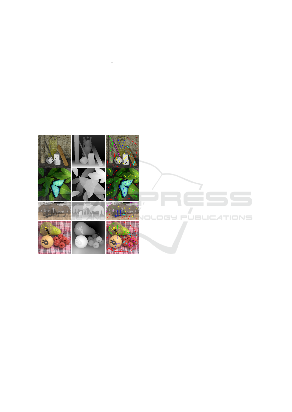
into several classes. In figure 1 it can be seen a view
for a fixed s and t and the depth math corresponding
to the same s and t. The number of classes are 7 for
the Horses dataset, 6 for the Buddha and Still Life
datasets and 4 for Papillon dataset.
Figure 1: Heidelberg database. In the first column we show
the central image (s = 5, t = 5) of 81 possible views of the
sets Buddha, Papillon, Horses and Still Life. In the second
column the depth image is used as a fourth channel. Third
column, scribbles used in the projection step.
To evaluate the method we use the percentage of
pixels well classified and the Jaccard similarity index,
which measures the overlap (agreement) between two
binary images X and Y, by taking the ratio between
the size of their intersection and the size of their
union: J(X,Y ) = |X ∩Y |/|X ∪Y |. This metric yields
values between 0 and 1, where 0 means complete dis-
similarity and 1 stands for identical images.
Although it is not required for the model, in this
experiment we used scribbles in the threshold step to
estimate the probability density function at each class
i as a multivariate Gaussian distribution defined by its
Table 1: Percentage of well classified pixels for the different
datasets (accuracy ratio).
Buddha 97.73 %
Papillon 98.37 %
Horses 97.39 %
Still Life 98.2 %
vectorial mean ¯µ
i
and its covariance matrix Σ
i
com-
puted from of u
∗
. Then
x ∈ Ω
i
⇐⇒ p
i
(u
∗
(x)| ¯µ
i
,Σ
i
) ≥ p
j
(u
∗
(x)| ¯µ
i
,Σ
i
), ∀ j 6= i
The scribbles we used for computing the mixture
Gaussian probabilities in the threshold step are shown
in figure 1. We would like to remark that although the
scribbles are drawn on the original image, the vec-
torial mean ¯µ
i
and the covariance matrix Σ
i
are esti-
mated from u
∗
.
The results are resumed in tables 1 and 2 and
shown in figure 2 where we show the computed parti-
tion (first column of figure 2) and the piecewise con-
stant function u = C
¯
χ (last column) produced by the
method. The parameter λ of the model was cho-
sen empirically with values λ = 0.674 for Buddha,
λ = 0.0554 for Papillon λ = 0.0765 for Horses and
λ = 0.0554 for Still Life. In the four tested datasets,
the accuracy ratio (table 1) is around 98% and the Jac-
card similarity index (table 2) goes from 0.7 to 0.99,
depending on the size of the region (class) consid-
ered. The accuracy results we obtained are compara-
ble with those in (Wanner et al., 2013b) being the dif-
ference less than 1% for Buddha, Papillon and Horses
datasets and around 0.3% for Still Life dataset. It is
worth to say that we have used less features than in
(Wanner et al., 2013b). In fact we use only the color
and the given depth while, in (Wanner et al., 2013b),
the eigenvalues of Hessian matrix has been used.
5 CONCLUSIONS
We have extended the Anisotropic Mumford-Shah
energy functional originally proposed by Osher and
Vese (Osher and Paragios, 2003) for the binary seg-
mentation of 2D gray color images to the general case
of multi-class segmentation of vectorial images of any
dimension. The extension has been done using the
formalism for the local or common inter-phases be-
tween classes to decompose the boundary of a spe-
cific region into curves that correspond to the edge be-
tween a region and its neighbours (regions). As a fur-
ther contribution, we proved the equivalence between
the proposed energy functional and the well known
A Multiclass Anisotropic Mumford-Shah Functional for Segmentation of D-dimensional Vectorial Images
473
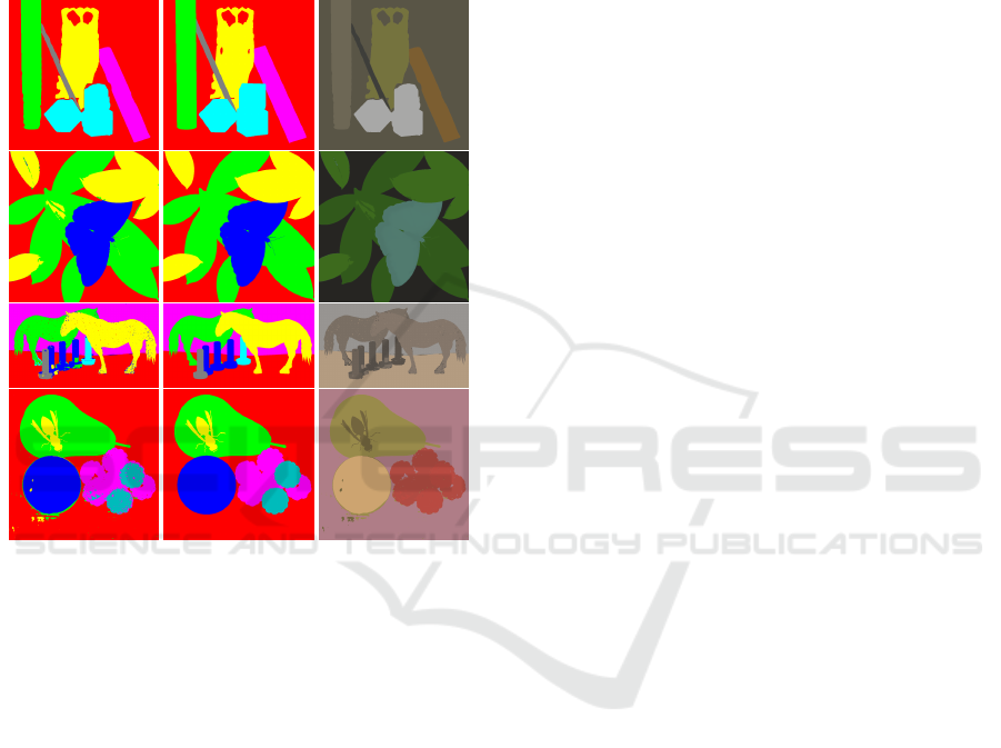
Table 2: Jaccard similarity index. Those datasets marked as ’-’ means that there is no class with this color.
Red Green Blue Yellow Cyan Pink Purple Gray
Buddha 0.96 0.95 - 0.96 0.95 0.94 - 0.81
Papillon 0.99 0.96 0.99 0.94 - - - -
Horses 0.98 0.93 0.73 0.96 0.84 0.98 - 0.88
Still Life 0.99 0.98 0.98 0.88 - 0.88 0.81 -
Figure 2: Results. First column shows the classes detected
for the central view (s = 5, t = 5). Second Column shows
the ground truth. Third Column shows the final piecewise
constant computed u in which the color corresponds to the
optimal constant.
Rudin-Osher-Fatemi denoising model when it is min-
imized over the piecewise constant function set. This
relationship allows us to rewrite the original problem
of segmentation, which is non-convex, as a convex
problem. Finally we show how to project the solu-
tions of the convex problem into the original space of
piecewise constant functions.
Convincing results were shown on the Heidelberg
Collaboratory group dataset, where the ground truth
is provided. Notice that depth information was added
as a feature in a new channel. This shows and ex-
emplifies how it is possible to use this general multi-
channel model for specific image modalities and tasks
processing. The accuracy of the results is around 96-
98% which is pretty good taking into account that
in comparison with other methods for LF image seg-
mentation, we use less features (color and depth).
ACKNOWLEDGEMENTS
The authors acknowledge partial support by
TIN2015-70410-C2-1-R (MINECO/FEDER, UE)
and by GRC reference 2014 SGR 1301, Generalitat
de Catalunya.
REFERENCES
Ambrosio, L., Fusco, N., and Pallara, D. (2000). Functions
of Bounded Variation and free discontinuity problems.
Clarendon Press, Oxford University.
Bresson, X. and Chan, T. (2008). Fast dual minimization of
the vectorial total variation norm and applications to
color image processing. Inverse Problems and Imag-
ing, 2(4):455–484.
Brown, E. S., Chan, T. F., and Bresson, X. (2011). Com-
pletely Convex Formulation of the Chan-Vese Image
Segmentation Model. International Journal of Com-
puter Vision, 98(1):103–121.
Chambolle, A. (2004). An Algorithm for Total Variation
Minimization and Applications. Journal of Mathe-
matical Imaging and Vision, 20(1/2):89–97.
Chambolle, A. and Darbon, J. (2008). On Total Variation
Minimization and Surface Evolution using Paramet-
ric Maximum Flows Antonin Chambolle and J
´
er
ˆ
ome
Darbon. International Journal of Computer Vision,
84(April):288–307.
Chambolle, A. and Lions, P.-L. (1997). Image recovery via
total variation minimization and related problems. Nu-
merische Mathematik, 76(2):167–188.
Chambolle, A. and Pock, T. (2011). A first-order primal-
dual algorithm for convex problems with applications
to imaging. In J. Math. Imaging Vision, volume 40,
pages 120–145.
Chan, T. F. and Vese, L. a. (2001). Active contours with-
out edges. IEEE transactions on image processing :
a publication of the IEEE Signal Processing Society,
10(2):266–77.
Garamendi, J. F., Gaspar, F. J., Malpica, N., and Schiavi,
E. (2013). Box relaxation schemes in staggered dis-
cretizations for the dual formulation of total variation
minimization. IEEE transactions on image process-
ing, 22(5):2030–43.
Klann, E. and Ramlau, R. (2013). Regularization Properties
of Mumford–Shah-Type Functionals with Perimeter
and Norm Constraints for Linear Ill-Posed Problems.
SIAM Journal on Imaging Sciences, 6(1):413—-436.
VISAPP 2017 - International Conference on Computer Vision Theory and Applications
474

Lippman, R. (1908). La photographie int
´
egrale. Acad
´
eemie
des sciences, pages 446–551.
Mumford, D. and Shah, J. (1989). Optimal approximations
by piecewise smooth functions and associated varia-
tional problems. Communications on Pure and Ap-
plied Mathematics, 42(5):577–685.
Ng, R. (2006). Digital light field photography. PhD thesis.
Ng, R., Levoy, M., Duval, G., Horowitz, M., and Hanrahan,
P. (2005). Light Field Photography with a Hand-held
Plenoptic Camera. Informational, pages 1–11.
Nikolova, M., Esedoglu, S., Chan, T. F., Esedo, S., and Glu,
. (2006). Algorithms for Finding Global Minimizers
of Image Segmentation and Denoising Models. SIAM
Journal on Applied Mathematics, 66(5):1632–1648.
Osher, S. and Paragios, N. (2003). Geometric level set meth-
ods in imaging, vision, and graphics.
Perwass, C. and Wietzke, L. (2010). www.raytrix.de.
Pock, T., Chambolle, A., Cremers, D., and Bischof, H.
(2009). A convex relaxation approach for computing
minimal partitions. In 2009 IEEE Computer Society
Conference on Computer Vision and Pattern Recogni-
tion Workshops, CVPR Workshops 2009, pages 810–
817.
Reddy, D., Bai, J., and Ramamoorthi, R. (2013). External
mask based depth and light field camera. Workshop
Consumer Depth Cameras for Vision.
Rousson, M. and Deriche, R. (2002). A variational frame-
work for active and adaptative segmentation of vector
valued images. In Proceedings - Workshop on Motion
and Video Computing, MOTION 2002, pages 56–61.
Institute of Electrical and Electronics Engineers Inc.
Rudin, L., Osher, S., and Fatemi, E. (1992). Nonlinear total
variation based noise removal algorithms. Physica D:
Nonlinear Phenomena, 60(1-4):259–268.
Wanner, S., Meister, S., and Goldluecke, B. (2013a).
Datasets and Benchmarks for Densely Sampled 4D
Light Fields. In Vision, Modeling \& Visualization,
pages 225—-226.
Wanner, S., Straehle, C., and Goldluecke, B. (2013b). Glob-
ally Consistent Multi-label Assignment on the Ray
Space of 4D Light Fields. 2013 IEEE Conference
on Computer Vision and Pattern Recognition, pages
1011–1018.
A Multiclass Anisotropic Mumford-Shah Functional for Segmentation of D-dimensional Vectorial Images
475
