LiDAR-based 2D Localization and Mapping System using Elliptical

Distance Correction Models for UAV Wind Turbine Blade Inspection

Ivan Nikolov and Claus Madsen

Department of Architecture, Design, and Media Technology, Aalborg University, Rendsburggade 14, Aalborg, Denmark

{iani, cbm}@create.aau.dk

Keywords:

Localization, Mapping, Scanning, LiDAR, IMU, UAV, SLAM, Wind Turbine Blades Inspection.

Abstract:

The wind energy sector faces a constant need for annual inspections of wind turbine blades for damage, erosion

and cracks. These inspections are an important part of the wind turbine life cycle and can be very costly and

hazardous to specialists. This has led to the use of automated drone inspections and the need for accurate,

robust and inexpensive systems for localization of drones relative to the wing. Due to the lack of visual

and geometrical features on the wind turbine blade, conventional SLAM algorithms have a limited use. We

propose a cost-effective, easy to implement and extend system for on-site outdoor localization and mapping in

low feature environment using the inexpensive RPLIDAR and an 9-DOF IMU. Our algorithm geometrically

simpliﬁes the wind turbine blade 2D cross-section to an elliptical model and uses it for distance and shape

correction. We show that the proposed algorithm gives localization error between 1 and 20 cm depending on

the position of the LiDAR compared to the blade and a maximum mapping error of 4 cm at distances between

1.5 and 3 meters from the blade. These results are satisfactory for positioning and capturing the overall shape

of the blade.

1 INTRODUCTION

As robots and drones become widely used in different

branches of the industry, a need for localization and

mapping systems, which are able to work in non-ideal

conditions, arises. The state of the art for drone simul-

taneous localization and mapping (SLAM) is most

widely used both from monocular (Mur-Artal et al.,

2015), stereo camera (Endres et al., 2012), LiDAR

and laser scanners (Berger, 2013) (Zlot and Bosse,

2014) . A lot of SLAM algorithms for the outdoors

are used together with GPS positioning and orienta-

tion from an inertial measurement unit (IMU) (Else-

berg et al., 2012) (Shepard and Humphreys, 2014).

SLAM algorithms work best in environments, which

are rich in geometric features and vary signiﬁcantly.

The precision of these algorithms signiﬁcantly suffers

when the environment is too featureless or when there

are insufﬁcient number of points of interest, which

requires the introduction of algorithm modiﬁcations,

such as visual feature clustering (Negre et al., 2016)

or combining camera and laser scanner depth data

(Oh et al., 2015). When the number of points ex-

tracted from laser scanner is too low, due to sharp cor-

ners or thin surfaces, these modiﬁcation cannot sus-

tain a high enough performance. Similar problems

are present when using drones in the wind energy sec-

tor for inspection of wind turbine blades. Wind tur-

bine blades are normally located at over 100 meter

heights and do not have any other landmarks around

them. This, combined with the monochrome color of

the blades and the lack of corners and other geometric

features, makes autonomous localization of the drone

and mapping the environment, hard.

We propose a cost-effective and easy to imple-

ment solution for localization and mapping the over-

Figure 1: Our proposed localization and mapping solution

using elliptical distance correction models.

418

Nikolov I. and Madsen C.

LiDAR-based 2D Localization and Mapping System using Elliptical Distance Correction Models for UAV Wind Turbine Blade Inspection.

DOI: 10.5220/0006124304180425

In Proceedings of the 12th International Joint Conference on Computer Vision, Imaging and Computer Graphics Theory and Applications (VISIGRAPP 2017), pages 418-425

ISBN: 978-989-758-227-1

all shape of the blade (Figure 1), designed to work in

feature-poor wind turbine blade environments, with

minimum prior information. Our system consists of

the RPLIDAR scanner and the BNO055 9-DOF IMU

for orientation. Our algorithm is based on the assump-

tion that a blade is stopped in a vertical position, at

either the top or bottom and is the only thing that is

visible for the LiDAR. The algorithm uses prior in-

formation for the cross-section width and depth and

it models the blade using primitive elliptical shapes,

providing drone positioning relative to the blade in

a much simpler way than conventional SLAM algo-

rithms. The initial angle between the LiDAR and

blade is found by using a 2D iterative closest point

(ICP) algorithm and the angle heading is monitored

and maintained using an IMU. Additionally we model

the distance measurement and sampling errors of the

RPLIDAR to boost the accuracy of the localization.

We address the sunlight noise problem of the RPL-

IDAR with a hybrid hardware and software ﬁltering

solution. We perform initial ground-based tests on

the system to determine its accuracy and error rate

by comparing with ground truth manually measured

positions. Additionally we estimate to what extent

the algorithm can capture the overall shape of the 2D

cross-section of the blade, using a ground truth cross-

section. Both tests demonstrate that the system per-

forms well even with a small number of points present

from the scanned area and can be used for drone local-

ization relative to the blade and generation of initial

sparse 2D point clouds of the shape of the blade.

2 STATE OF THE ART

Drone inspection of wind turbine blades is a hot

topic for the computer vision, automaton and robotics

ﬁelds. The limited number of points of interest, the

featureless and monochrome shape of the wind tur-

bine blades and the required operational height, to-

gether with environment hazards like gusts of wind,

blade swaying and weather changes make localiza-

tion and mapping non-trivial problems. The research

from (Morgenthal and Hallermann, 2014) shows that

inspection by images can suffer signiﬁcantly if the

drone’s localization and stabilization systems cannot

compensate for environmental and weather changes.

One way to tackle these problems is to have an initial

ﬂy-through, through which an occupancy map of the

blade is created and which is then used for planning

a ﬂightpath, as suggested by (Sch

afer et al., 2016).

Another solution proposed by (Jung et al., 2015) can

come not only from relying on a ﬂying drone, but

creating a hybrid ﬂying and climbing vehicle, which

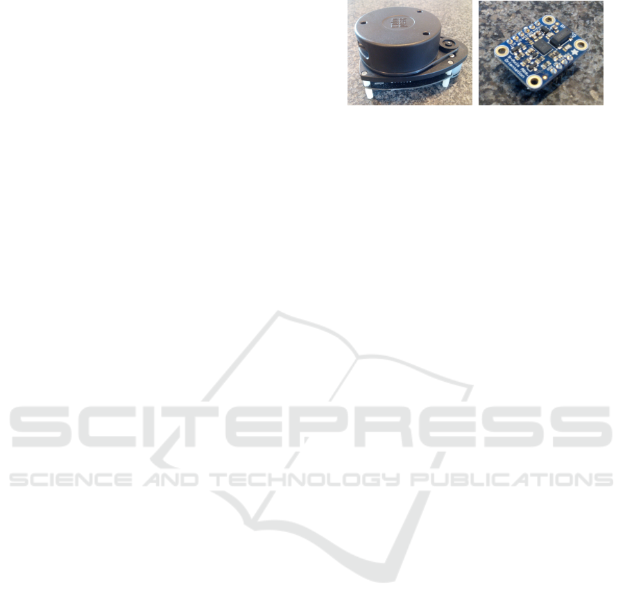
(a) (b)

Figure 2: The hardware used for the proposed system - the

RPLIDAR and the BNO055 9-DOF IMU.

uses a combination of sonar, IMU and LiDAR system

to orient itself. Using a dynamic ﬂightpath planning

from a camera feed is a another strategy employed by

(Galleguillos et al., 2015) and (Cordero et al., 2014),

combining it together with navigation sensors like an

IMU, GPS, barometer, etc.

We propose a localization and shape mapping sys-

tem, which uses a LiDAR scanner and an IMU, plus a

simpliﬁcation of the wind turbine blade cross-section

to a elliptical model for distance and shape correc-

tion. Our algorithm is based on the assumption that

only the blade is visible at any time and works even

when as little as 2 or 3 points are obtained from the

scanned surface.

3 METHODOLOGY

3.1 Algorithm Overview

The proposed system, given in Figure 3, relies on

prior shape information for a proper positioning. The

prior information in our case, comes in the form of

a model of the shape of the blade cross-section. Be-

cause ﬁnding a real world 3D model for each piece of

the cross-section of the different kinds of blades in a

problematic task, a simpliﬁed elliptical model is pro-

posed. The elliptical model requires much less prior

information and it gives centimeter precision results

as shown in Section 4. Stray sunlight in the sensor

causes detection noise, which is ﬁltered away using a

combination of hardware polarization and software k-

nearest neighbors and line ﬁlters, before the LiDAR’s

raw data is used.

As an initial step, before the main localization al-

gorithm is started, the angle between the blade and

drone is calculated using readings from a low-cost Li-

DAR from (Slamtec, 2010), shown in Figure 2a and

an 2D iterative closest point algorithm, as described

in Subsection 3.4. The angle is used to rotate the el-

liptical model in the same direction as the blade and is

then maintained with the readings from the IMU from

(Adafruit, 2012), shown in Figure 2b. It is observed

LiDAR-based 2D Localization and Mapping System using Elliptical Distance Correction Models for UAV Wind Turbine Blade Inspection

419

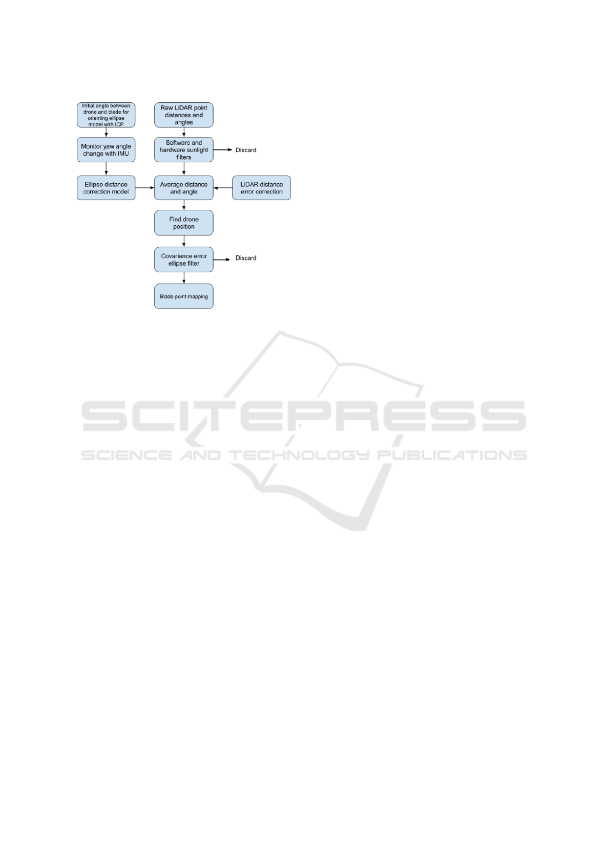
Figure 3: Algorithm and work pipeline overview. From raw

LiDAR data and IMU orientation, to localization of the Li-

DAR compared to the blade and mapping the points of the

blade cross-section.

that the LiDAR exhibits errors in its readings, which

change with the distance from the measured surface.

To compensate for this error, we compare the mea-

surements from the LiDAR and ground truth readings

from a DISTO laser distance scanner. The differences

are calculated, interpolated and smoothed out using a

cubic spline and used as distance corrections.

Once the data is clear of noise, corrected from

the distance errors and properly rotated, the ellipti-

cal distance correction model (EDC model) as seen

in Subsection 3.3, together with the angle correction

from the IMU, are applied. The localized drone po-

sition is ﬁltered to remove false movement readings

using a covariance ellipse error ﬁltering, as proposed

by (Friendly, 1991) and the blade points are mapped

accordingly.

3.2 From Corrected LiDAR Data to

Initial Drone Localization

The corrected output data from the RPLIDAR comes

in polar coordinates. To position the data for each Li-

DAR reading in a uniﬁed coordinate system, the data

is ﬁrst transformed to Cartesian coordinates. We as-

sume that only the wind turbine blade is seen by the

LiDAR at any given time, so the origin of the new

Cartesian coordinate system is chosen to be the cen-

ter of the scanned blade. We then wish to map ev-

erything to this coordinate system - both drone po-

sitions and blade surface points. Formula 1 is used

for transforming the coordinates. Lets for a moment

also assume that the centroid of the measured points

from the LiDAR is a good approximation for the cen-

ter of te blade, independent of where the LiDAR is

compared to the blade. Naturally the are problems

with that assumption and we will demonstrate how to

compensate for that error in the next sections.

= 0 − D

mean

· sin(α

mean

)

= 0 − D

mean

· cos(α

mean

)

(1)

Where the x

and y

are the drone coordinates in

the new coordinate system, D

mean

and α

mean

are the

mean distance and angle calculated from all detected

points in a 360 degree reading. Once the LiDAR is

self localized, compared to the blade, the LiDAR’s

position is used as a new center of a polar coordinate

system to ﬁnd the blade’s previously detected points.

The points are calculated in a Cartesian coordinate

system using Formula 2.

= x

+ D

· sin(α

)

= y

+ D

· cos(α

)

(2)

Here x

and y

, are the coordinates of each of the

data points in one reading and D

and α

are respec-

tively their distances and angles. The center for calcu-

lating the blade points positions is the LiDAR’s coor-

dinates x

and y

, calculated in Formula 1. The whole

process is visualized in Figure 4. The initial naive ap-

proach to localization and mapping yields some prob-

lems, such that the whole cross-section needs to be

opened up. Additional processing is required to get

the correct cross-section mapping and position local-

ization. This is why we introduce the elllipse distance

correction model (EDC model).

3.3 Elliptical Distance Correction

Model (EDC Model)

In real life the LiDAR does not measure the distance

from the drone to the blade center, but to the exterior

shell/body of the blade. The distance from the cen-

ter of the blade to the exterior points that the LiDAR

measures is not known to the LiDAR. This discrep-

ancy leads to improper modeling of the surface shape

of the blade and incorrect drone position calculation.

To be able to capture the proper shape of the blade

proﬁle and the proper LiDAR positions, an initial

guess of the blade form is needed. The wing of a

wind turbine has a very speciﬁc and hard to model

shape, which changes with height. Each blade man-

ufacturer has different speciﬁcations, numbering and

shape mold and this information is not readily avail-

able. Therefore, an approximate simpliﬁed model is

VISAPP 2017 - International Conference on Computer Vision Theory and Applications

420

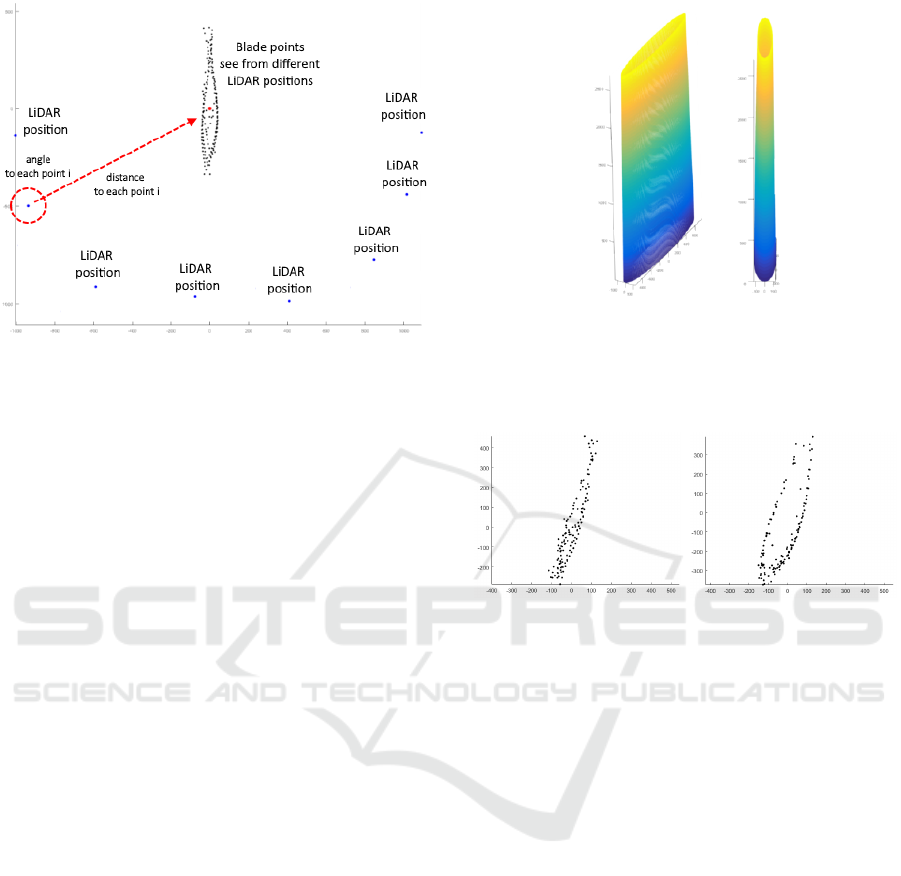
Figure 4: Initial drone localization. The corrected LiDAR

data is transformed into a Cartesian coordinate system and

the mean angle and distance are used to self-position the

LiDAR compared to the blade. Once these positions are

found they are used to ﬁnd the blade points’ positions. Eight

LiDAR positions and the visible blade points are plotted in

the Figure.

required as a substitute of the blade shape. The model

can be further adjusted using known blade shapes.

This requires making some assumptions:

• The LiDAR sees only the wind turbine blade;

• The wind turbine blade is stopped;

• The blade’s cross-section width and depth are

known;

• The vertical position of the drone is known.

An ellipse is suggested as such a simple geometri-

cal shape, as it closely resembles the the blade cross-

section, especially in the leading edge. To model

properly the blade’s size for the different heights, an

ellipse shape is calculated for each height slice of the

blade. The ellipse points are calculated using the For-

mula 3, where r

and r

are the two radii of the ellipse,

which are selected based on the width and depth of

the cross-section at the particular blade height and the

angle β ∈ [0 : 2π] .

= 0 − r

· sin(β)

= 0 − r

· cos(β)

(3)

A full model of the blade is created and is saved in

a table, for an easy access depending on the height of

the drone, compared to the blade. Multiple elliptical

models can be created for different blade dimensions

and manufacturer models. A full 3D model can be

seen in Figure 5.

For each point on the ellipse, the radius from the

center to the point is calculated, as well as the angle

on a circle with a center in (0,0). Each point on the

Figure 5: Elliptical model for correcting the LiDAR’s po-

sition. The 3D model is created with interpolation of the

two radii of the ellipse cross-section in Z direction, follow-

ing the notion that wind turbine blades become smaller with

height.

(a) Without EDC model (b) With EDC model

Figure 6: Example mapping of the blade before and after

the EDC model. The points’ positions are corrected and the

whole proﬁle is opened up, especially the blade edge points.

ellipse is positioned in the same coordinate system as

the points from the LiDAR. This way when the Li-

DAR position is calculated using the mean distance,

the distance of the point on the ellipse with the closest

angle to the mean angle of the LiDAR is added to it.

This effectively pushes outwards the mean points and

gives an initial guess on the shape of the blade. The

difference can be seen when plotting the blade sur-

face points before and after the elliptical correction,

as seen in Figure 6. The correction is most notice-

able on the points on the leading edge of the blade.

The whole proﬁle is opened up, representing the blade

cross-section more closely.

Another problem becomes evident when using the

EDC model - the ellipse needs to be initially oriented

the same way as the blade proﬁle. The rotation of the

blade is initially unknown and needs to be determined

before the correction can be applied to the localization

and mapping.

LiDAR-based 2D Localization and Mapping System using Elliptical Distance Correction Models for UAV Wind Turbine Blade Inspection

421

3.4 Calculating Initial Angle between

Drone and Blade

The drone’s yaw orientation is taken from the IMU

unit. The angle between the detected blade proﬁle

from the LiDAR and the IMU connected to the drone

is calculated. The initial angle is used to ﬁrst orient

the ellipse compared to the blade’s orientation for the

EDC model and also for keeping the mapped posi-

tions at the same heading. The change in the orien-

tation of the wind turbine blade, while the LiDAR is

scanning, is deemed too small, as it will be stopped

from moving or rotating for the duration of the drone

ﬂight.

The angle between the blade and LiDAR can be

calculated using ICP. Heuristically it is determined

that at least 8 points are required in one reading for

the ICP registration to be successful. The sides of

the blade are better for registration than the edge,

as they contain more points, which are spread more

evenly. Because the success of the ICP depends on

the quantity and quality of the registration points, a

cubic spline is approximated to the scanned points.

This way the scanned points are interpolated and any

small noise position errors are smoothed over. A 2D

ICP algorithm by (Bergstr

om and Edlund, 2014) is

used to register the LiDAR points to the prior ellip-

tical model. A rigid registration is performed with

only rotation and translation, as the ellipse is properly

sized beforehand, using the initial information for the

width and depth of the blade proﬁle. The process can

be seen in Figure 7.

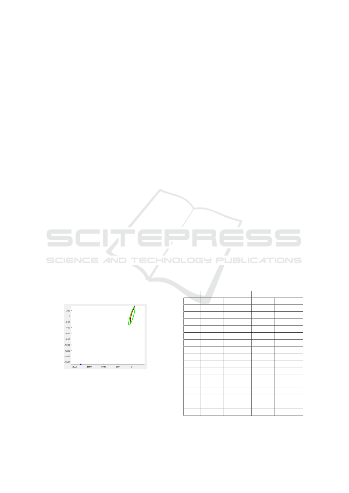
Once the registration is completed, the rotation an-

gle is used to rotate the EDC model. The angle is also

added to the yaw angle measured by the IMU for use

with the drone’s yaw holding.

Figure 7: Initial ICP orientation of the EDC model. Blue

points show the LiDAR’s reading, red points are the approx-

imated cubic spline and the green ellipse is the correction

model.

4 SYSTEM TESTS AND RESULTS

4.1 Localization Test

The ﬁrst test aims to measure the localization accu-

racy of ﬁnding the position of the LiDAR compared

to the blade. As the system is still in the prototyping

stages, the measurements are done on the ground. A

number of ground truth points are measured around

the blade proﬁle, ranging from 0.5m to 3.5m in dis-

tance from LiDAR to the blade leading edge. Two

sets of ﬁfteen positions are selected. The ﬁrst set is

with positions arranged in a circle and the second -

in a line. These are selected, to demonstrate the sys-

tem’s performance with different scan patterns. Both

sets contain outliers positions to verify the accuracy of

the system in harder localization points, such as those

far away or too close to the blade. The LiDAR is posi-

tioned on each of the ground truth points and the mea-

sured position is computed. Fifty readings are taken

so any noisy measurements can be ﬁltered away using

the covariance ellipse error ﬁltering. The Euclidean

distance between each of the ground truth positions

and measured LiDAR self positioning is computed,

both with and without the elliptical distance correc-

tion model. The resultant error values from the ﬁrst

and second position datasets are given in Table 1 and

the plotted LiDAR and blade points are given in Fig-

ure 8.

Table 1: Results from the ﬁrst and second set of posi-

tions around the blade. The distance error(mm) between the

ground truth position and the one measured by the LiDAR

with the correction algorithm E

algorithm

and with only the

raw data E

raw

Dataset 1 Dataset 2

Pos E

raw

algorithm

raw

algorithm

1 88.36 76.01 213.10 119.22

2 259.96 210.01 183.81 79.88

3 187.54 119.01 221.20 111.19

4 221.32 118.63 199.42 88.59

5 228.45 104.67 221.51 75.40

6 386.52 81.49 372.17 153.79

7 263.29 64.54 333.90 64.49

8 152.99 16.18 306.11 41.51

9 84.32 12.20 276.03 43.08

10 47.17 18.26 150.44 66.08

11 138.62 42.21 136.81 18.49

12 341.87 51.91 110.82 45.54

13 183.16 135.09 75.77 34.39

14 180.57 110.27 131.25 36.79

15 285.28 84.67 248.22 4.59

Avg 203.30 83.01 212.04 65.54

VISAPP 2017 - International Conference on Computer Vision Theory and Applications

422

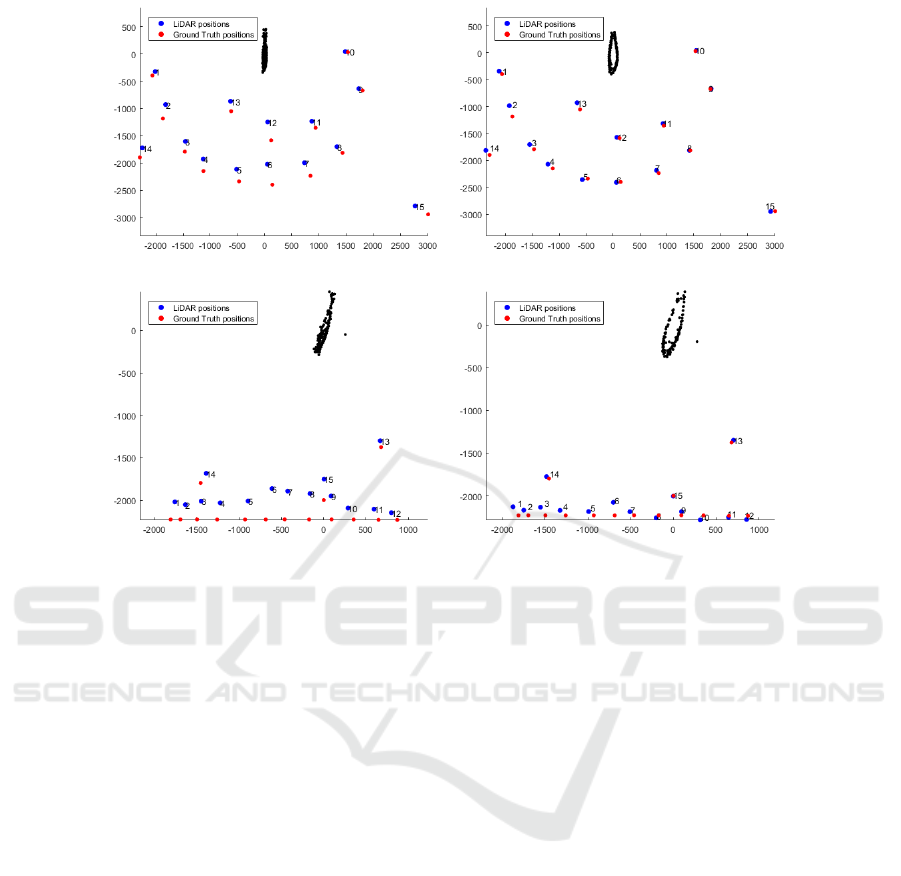
(a) Dataset 1 without EDC model (b) Dataset 1 with EDC model

Figure 8: Localization test using the ﬁrst (8a and 8b) and second(8c and 8d) position datasets. The ground truth data is

shown with red dots and the LiDAR calculated positions with blue dots. The mapped blade points are also plotted, for easier

orientation.

The results show that the system can provide a

stable position estimate for where the drone is com-

pared to the blade. The biggest differences between

the measured and ground truth points come from po-

sitions where just a small amount of points from the

surface can be seen in the Dataset 1 distances between

ground truth and measurements in positions 3, 4, 5

and 13. In addition positions which are too far away

from the blade surface exhibit both lower precision

and accuracy, because insufﬁcient points are sampled

by the LiDAR, which makes faraway point angle and

distance estimation jump around too much, as seen in

the measurement in position 14 and 15 in Dataset 1.

Some larger distances are observed in the ﬁrst dataset,

which can also be explained by problems with the

yaw hold and small changes in the rotation of the Li-

DAR, as seen in position 2. In all positions, the intro-

duction of the EDC model is shown to dramatically

increase the accuracy of the localization, compared to

just using the raw data. This is especially evident in

the measurements 5 to 9 from Dataset 2.

4.2 Mapping Test

For testing the mapping capabilities of the LiDAR

system, the blade proﬁle is scanned with a Faro laser

scanner and a high quality point cloud is created.

A 2D cross-cut of the point cloud is then used as a

ground truth, when comparing with the mapped blade

point positions. In this test the LiDAR is placed in

positions, forming a semicircle around the blade with

three radii - 1.5 m, 2 m and 3 m, for testing the map-

ping capabilities from different distances. Addition-

ally a post-processed mapping from 1.5 m, which has

been registered to the elliptical prior model using the

ICP algorithm is given, to demonstrate one way that

the proposed algorithm can be extended to boost ac-

curacy. The signed distances between each point of

the two 2D point clouds is calculated. This is done

using the free open source software CloudCompare

(Girardeau-Montaut, 2003). From the distances, the

mean and standard deviation of the distance distribu-

tion are calculated. The mean and standard deviation

are given in Table 2 and the mapped blade surface

points are given in Figure 9

The difference between the elliptical correction

model and the blade cross-section becomes larger the

farther away from the edge it goes, because the scan-

ning is done only in a 180 degree semi-circle around

the blade and details of the back of the blade are

sparse. The front of the blade in the LiDAR scans

shows a higher standard deviation and some noisy

LiDAR-based 2D Localization and Mapping System using Elliptical Distance Correction Models for UAV Wind Turbine Blade Inspection

423

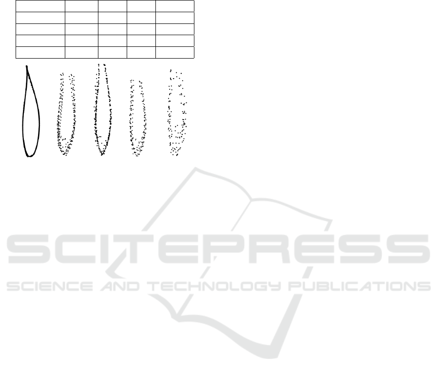
Table 2: Mean value (µ) in mm, standard deviation (σ) in

, minimum (d

min

) and maximum (d

max

) in mm of the

absolute distance metrics between the ground truth and the

LiDAR mapped points from three distances to the blade

) - 1.5, 2 and 3 meters.

µ σ d

min

max

1.5 10.93 7.32 0.36 38.13

1.5 + ICP 9.32 6.92 0.24 31.038

2 14.89 9.19 0.62 38.40

3 15.65 9.23 1.31 39.30

(a)

Ground

truth

(b) 1.5

meters

+ ICP

(d) 2

meters

(e) 3

meters

Figure 9: Mapped blade surface from the LiDAR, using the

EDC model, together with the ground truth Faro scan and

the post-processed 1.5 meter mapping using the ICP algo-

rithm together with the elliptical prior model. The 2D point

clouds get sparser and noisier the further away the LiDAR

is.

points, because of the small amount of points seen

from those angles. Even with these problems and the

relatively small sampling density of the RPLIDAR,

the proposed algorithm manages to restore the shape

of the blade with centimeter accuracy. If a registra-

tion is done, the results get closer to the ground truth

shape. This shows that the algorithm can be used as a

proper substitute to SLAM.

5 CONCLUSION AND FUTURE

WORK

We propose a low-cost, easy to implement drone

localization and mapping system for wind turbine

blades, using a cheap commercial LiDAR and an off-

the-shelf IMU. Our system uses prior shape infor-

mation in the form of elliptical distance correction

model. It requires minimum prior information; it is

computationally fast; simpler to implement than con-

ventional SLAM; it can easily be extended and reﬁned

with additional training and provides satisfactory re-

sults. We demonstrate through ground based localiza-

tion and a mapping tests that the system can self po-

sition and obtain mapping of the blade cross-cut with

centimeter accuracy. In addition we propose a ﬁlter

for removing noisy position information. Our algo-

rithm also removes distance measurement errors and

direct sunlight noise, so it can be used both outdoors

and indoors.

As an extension of our work we propose an in-

depth test of our system and algorithm against the

state of the art SLAM algorithms performed on blade

proﬁles, to verify the calculated accuracy of the sys-

tem. Testing the algorithm using a ”default” blade

shape, which will better resemble the scanned blades,

as a distance correction model is also suggested, as

well as further adjusting it using training sets.

REFERENCES

Adafruit (2012). Adafruit bno055 9-dof imu. https://learn.

adafruit.com/adafruit-bno055-absolute-orientation-

sensor. Accessed: 2016-09-15.

Berger, C. (2013). Toward rich geometric map for slam:

Online detection of planes in 2d lidar. Journal of Au-

tomation Mobile Robotics and Intelligent Systems, 7.

Bergstr

om, P. and Edlund, O. (2014). Robust registra-

tion of point sets using iteratively reweighted least

squares. Computational Optimization and Applica-

tions, 58(3):543–561.

Cordero, M., Trujillo, M., Ruiz, J., Jimenez, A., Diaz,

L., and Viguria, A. (2014). Flexible framework for

the development of versatile mav systems for multi-

disciplinary applications. In IMAV 2014: Interna-

tional Micro Air Vehicle Conference and Competition

2014, Delft, The Netherlands, August 12-15, 2014.

Delft University of Technology.

Elseberg, J., Borrmann, D., and N

uchter, A. (2012).

6dof semi-rigid slam for mobile scanning. In 2012

IEEE/RSJ International Conference on Intelligent

Robots and Systems, pages 1865–1870. IEEE.

Endres, F., Hess, J., Engelhard, N., Sturm, J., Cremers, D.,

and Burgard, W. (2012). An evaluation of the rgb-

d slam system. In Robotics and Automation (ICRA),

2012 IEEE International Conference on, pages 1691–

1696. IEEE.

Friendly, M. (1991). SAS system for statistical graphics.

SAS Publishing.

Galleguillos, C., Zorrilla, A., Jimenez, A., Diaz, L., Mon-

tiano,

A., Barroso, M., Viguria, A., and Lasagni, F.

(2015). Thermographic non-destructive inspection of

wind turbine blades using unmanned aerial systems.

Plastics, Rubber and Composites.

Girardeau-Montaut, D. (2003). Cloudcompare. http://

www.cloudcompare.org/. Accessed: 2016-09-15.

Jung, S., Shin, J.-U., Myeong, W., and Myung, H. (2015).

Mechanism and system design of mav (micro aerial

vehicle)-type wall-climbing robot for inspection of

wind blades and non-ﬂat surfaces. In Control, Au-

tomation and Systems (ICCAS), 2015 15th Interna-

tional Conference on, pages 1757–1761. IEEE.

VISAPP 2017 - International Conference on Computer Vision Theory and Applications

424

Morgenthal, G. and Hallermann, N. (2014). Quality assess-

ment of unmanned aerial vehicle (uav) based visual

inspection of structures. Advances in Structural Engi-

neering, 17(3):289–302.

Mur-Artal, R., Montiel, J., and Tard

os, J. D. (2015). Orb-

slam: a versatile and accurate monocular slam system.

IEEE Transactions on Robotics, 31(5):1147–1163.

Negre, P. L., Bonin-Font, F., and Oliver, G. (2016).

Cluster-based loop closing detection for underwater

slam in feature-poor regions. In 2016 IEEE In-

ternational Conference on Robotics and Automation

(ICRA), pages 2589–2595. IEEE.

Oh, T., Kim, H., Jung, K., and Myung, H. (2015). Graph-

based slam approach for environments with laser scan

ambiguity. In Ubiquitous Robots and Ambient Intel-

ligence (URAI), 2015 12th International Conference

on, pages 139–141. IEEE.

Sch

afer, B. E., Picchi, D., Engelhardt, T., and Abel, D.

(2016). Multicopter unmanned aerial vehicle for au-

tomated inspection of wind turbines. In 2016 24th

Mediterranean Conference on Control and Automa-

tion (MED), pages 244–249. IEEE.

Shepard, D. P. and Humphreys, T. E. (2014). High-precision

globally-referenced position and attitude via a fusion

of visual slam, carrier-phase-based gps, and inertial

measurements. In 2014 IEEE/ION Position, Loca-

tion and Navigation Symposium-PLANS 2014, pages

1309–1328. IEEE.

Slamtec (2010). Slamtec rplidar. http://

www.slamtec.com/en. Accessed: 2016-09-15.

Zlot, R. and Bosse, M. (2014). Efﬁcient large-scale 3d

mobile mapping and surface reconstruction of an un-

derground mine. In Field and service robotics, pages

479–493. Springer.

LiDAR-based 2D Localization and Mapping System using Elliptical Distance Correction Models for UAV Wind Turbine Blade Inspection

425